3D Sound and Auralization

3D Audio

“3D audio” is a generic term covering systems that aim to deliver a spatially enhanced auditory display — the perceptual sense that sounds occupy positions around the listener, not just on a stereo line between two loudspeakers. Many other terms have been used commercially and technically (“surround,” “binaural,” “immersive,” “object-based,” “spatial,” “ambisonic,” …), but all are related in this aim. Once a research-laboratory technique, 3D audio is now mainstream: Dolby Atmos in cinemas and streaming, Apple Spatial Audio with personalised HRTFs in AirPods, ambisonic delivery in VR/AR, and dynamic head-tracked binaural rendering in games and conferencing tools. The remaining frontiers are in personalisation (per-listener HRTFs), motion-aware rendering (head and body tracking), and low-latency interactive auralisation — not basic feasibility. The ambisonic methods named here encode a whole sound field as spherical harmonics; those first- and higher-order building blocks — the three-dimensional generalization of the microphone directivity patterns from Chapter 5 — can be explored in the Spherical Harmonics Explorer. The order is not a quality setting so much as a size one: a first-order recording reconstructs the field accurately across a head-sized region only up to about 600 Hz, third order to roughly 1.8 kHz, and seventh to 4.2 kHz, at a cost of 4, 16, and 64 channels respectively. Why that is comes down to which side of the sphere the sources are on.

Nominally, we would describe a sound in terms of three perceptual categories: pitch, tone color, and loudness; or in terms of their equivalent physical descriptors, frequency, spectral content, and intensity. However, spatial location is also an important perceptual quality. It’s the ability to manipulate spatial location that defines the “3D” aspect of spatial-audio technology.

How do we hear sounds in space? For a long time, researchers held that interaural intensity and interaural time differences were the cues used for auditory localization. For instance, a finger snap to the right of the head arrives with greater intensity at the right ear than at the left. Higher frequencies are shadowed from the opposite ear by the head; but frequencies below about 1.5 kHz diffract around to the opposite ear. The overall difference in intensity levels at the two ears are interpreted as changes in the sound source position from the perspective of the listener. This is the same cue used by the pan control on a mixer; by adjusting the output level between left and right speakers, it is possible to manipulate the perceived spatial location of the virtual image. Note that when the signal level is equal from both speakers and we’re listening from a position between them, the signal appears at a virtual position between the speakers, rather than as two sounds in either speaker.

Another cue for spatial hearing besides the interaural intensity difference is the interaural time difference. The wavefront reaches the right ear before the left ear in time, since the path length to that ear is shorter, and sound travels at a constant rate through air. These differential arrival times are also evaluated as a cue to the change of a sound source’s position. Wearing headphones and using a digital delay applied to the left channel, a sound file of a finger snap can be made to travel from the center of the head to the right side, by increasing the inter-channel delay from 0 to about 1 millisecond. This time delay cue is most effective for lower frequencies below 1.5 kHz.

Effects produced like this over headphones are not really localized as much as they are lateralized. This refers to spatial illusions that are heard inside or at the edge of the head, but never seem at a distant point outside the head, or externalized. Why aren’t these sounds externalized if we’re activating important spatial cues of interaural time and intensity differences? There are three reasons. The first is the lack of proper feedback from head motion cues. When we hear a sound we wish to localize, we move our heads in order to minimize the interaural differences, using our heads as a sort of pointer. This makes sense because we usually use our aural and visual senses together, and we’d want to look at the thing we’ve localized via sound (probably to decide whether to pounce or run, “fight or flight” from an evolutionary perspective). With headphone listening, head movement causes no change in spatial auditory perspective — it remains invariant, no matter where the head is. Head movement in relationship to stereo loudspeakers outside the head is even worse because intensity and time differences change with no relationship to the intended virtual imagery.

Another reason for imperfect localization with only intensity and time differences has to do with the spectral modification caused by the outer ears (the pinnae). This spectral modification can be thought of as equivalent to what a graphic equalizer does — emphasizing some frequency regions while attenuating others. The modification at one ear for a given position is technically referred to as the head-related transfer function (HRTF), sometimes also known as anatomical transfer function (ATF). This spectral modification has been recognized as an important cue to spatial hearing, especially for front-back or up-down cues.

Consider a sound source at right 60° azimuth, 0° elevation, along with another at the same elevation but at a “mirror image” position of right 120° azimuth. These two sound sources have roughly the same overall interaural time and intensity differences, as shown in Figure 9.1. On comparison, the rearward sound has a relatively “duller” timbre. In fact, for a given broadband sound source, each elevation and azimuth position relative to the listener contains a unique set of HRTF-based spectral modifications that act as an acoustic “thumbprint,” as shown in Figure 9.2. This is explained by the complex construction of the outer ears, which impose a set of minute delays that collectively translate into a particular two-ear (binaural) HRTF for each sound source position.

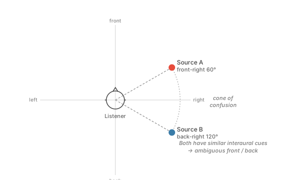
Figure 9.1. Two source positions on opposite sides of the front–back “cone of confusion” (red = front; blue = rear), at mirror-image azimuths around the interaural axis. Because they share nearly the same interaural time and intensity differences, the listener can confuse the front position with its rear twin — an ambiguity HRTF spectral cues are needed to resolve.

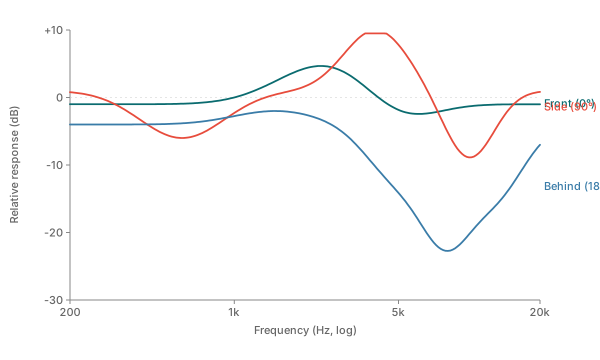
Figure 9.2. HRTF frequency modification for three positions. Inset: overhead view.

The final reason has to do with reverberation. Research implies that a virtual sound source is more effectively externalized over headphones when reverberation is present in the stimuli. In fact, there have been efforts over the last two decades to apply the same 3D sound techniques to reflected as well as direct sound, using ray tracing models of enclosures. This is termed auralization in acoustical design applications, and spatial reverberation in recording engineering applications.

There is a fourth reason, and the demonstrations on this page are subject to it. An HRTF is a measurement of one particular head: the folds of that listener’s outer ears, the width of that skull, the reflections from those shoulders. The spectral notches that distinguish above from below, and front from behind, sit at frequencies peculiar to the individual. Filtering with someone else’s measurement — a generic or non-individualized HRTF, which is what a browser, a game console, or this page provides — delivers the interaural time and intensity differences faithfully, since those depend mostly on head size, while placing the spectral cues in the wrong places. The usual result is exactly the weakness described above: sources that stay inside the head, elevations that refuse to separate, and a front position that keeps swapping with its rear twin. An individualized HRTF, measured on the listener in an anechoic chamber, largely removes these faults, and remains too laborious to be ordinary. The intermediate approaches — choosing a nearest match from a database by ear or by photographs of the ear, or warping a generic set towards the listener’s anatomy — are an active field precisely because the gap between generic and individualized is so audible.

In summary, there are three important cues for synthesizing a sound source to a given virtual position outside a headphone listener: (1) overall interaural level differences; (2) overall interaural time differences; and (3) spectral changes caused by the HRTF. Finally, it’s important to recognize that spatial hearing occurs within an environmental context, which is cued via unique patterns of reverberation.

Figure 9.3 places one source against one listener: a single sink — a single point of view. A natural extension is to place multiple sources and multiple sinks in the same scene, each with its own location, orientation, directivity, and audibility state. The second author’s paper “Exclude and Include for Audio Sources and Sinks: Analogs of Mute & Solo Are Deafen & Attend” (Presence 9:1, 2000) introduces the narrowcasting generalization: just as mute and solo selectively block or focus on individual sources, the symmetric operations deafen and attend selectively block or focus on individual sinks. Figure 9.4 is an interactive sandbox of that model.

Capturing and Synthesizing Spatial Audio

Spatial HRTF effects can be captured for a fixed listening position by use of a dummy head recording (see Figure 9.5). These mannequin heads contain a stereo microphone pair located in a position equivalent to the entrance of the human ear canal. A spatial recording can be obtained with such a device, but it is then difficult to move a particular virtual image to an arbitrary spatial position during post-production. What if we wanted 3D control over spatial imagery, instead of a pan control?

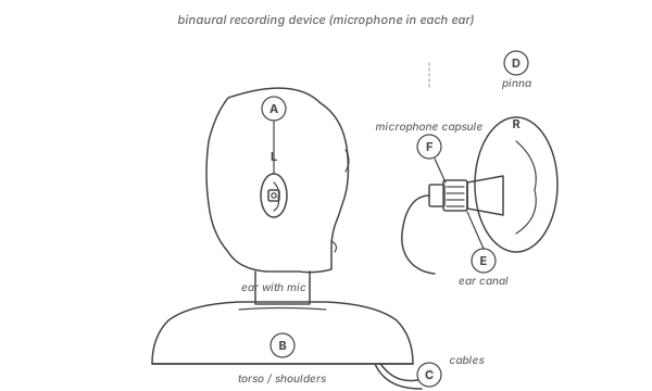
Figure 9.5. The HEAD Acoustics Model HMS II dummy head recording device. The outer ears were designed according to a “structural averaging” of HRTFs; note the inclusion of the upper torso.

This limitation is overcome through the use of 3D sound DSPs, both onboard and outboard. Without going into details (see the first author’s book 3-D Sound for Virtual Reality and Multimedia for that!), it is sufficient to know that HRTF measurements can be taken at various positions, which are then represented as digital filter parameters. These parameters can then be selectively recalled into 3D sound DSP units, depending on what position one wishes to simulate. By filtering an audio file or streamed or live source with the HRTF filter pairs (one for each ear), any spatial position can be simulated for a listener. Several research and development efforts are underway worldwide where HRTF measurements are collected, and subsequently utilized for digital filtering; 3D sound processing is part of several software packages. Although many of these efforts are commercial, some research programs also focus on perception, i.e. how much error is involved in the simulation.

That architecture — a bank of measured filter pairs, chosen by position — remains the core of binaural rendering, but it is no longer where most of the work is done. A spatial scene is now more often handed to the system as objects carrying positions, or as a sound field decomposed into spherical-harmonic (Ambisonic) components, and the filter pair is chosen by a renderer inside a game engine, an operating system, or the headphones themselves — many times a second, rather than once per configured source. The measurement and the filtering are unchanged; what moved is where the choice is made, and how often. The two descriptions answer different questions, and are worth keeping apart: Ambisonics represents the sound field itself, while binaural rendering is one of the ways that field can be delivered to a listener — the endpoint, not the representation.

Which renderer, and to what, is a separate question from how the scene was described. Over headphones the answer is the binaural one above. Over loudspeakers there are three broad families. Amplitude panning shares one source between the nearest speakers by gain alone; its general form, VBAP (vector base amplitude panning), picks the two or three speakers surrounding the wanted direction and solves for their gains, which is how most surround and dome rigs place a source. Ambisonics instead stores the field in spherical-harmonic components and decodes it to whatever speaker layout is present, first-order using four channels and higher-order using more, with directivity sharpening as the order rises — the reason the Spherical Harmonics Explorer is worth a visit here. Wave field synthesis, sometimes called holophony, is the most literal: a dense array of drivers reconstructs the wavefront itself, so the image stays put as a listener walks about, at the cost of needing tens or hundreds of channels. Over loudspeakers the binaural approach is also available, provided each ear can be given its own signal — which is the cross-talk cancellation described below. That technique is sometimes marketed as transaural; the word is a trademark, so cross-talk cancellation or loudspeaker binaural is the safer name in writing.

Figure 9.6 summarizes the aspects of spatial hearing that can be potentially manipulated by a 3D audio system, including azimuth, elevation, and distance of the virtual sound source. Simulation of environmental context is another aspect of virtual acoustic simulation; and finally, it would be ideal if we could arbitrarily control the virtual image’s size and extent. In reality, all of these factors interact, making absolute control over 3D audio imagery technically challenging.

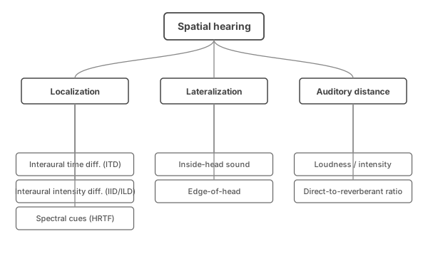
Figure 9.6. A taxonomy of spatial hearing.

Loudspeaker Playback of 3D Sound

Why doesn’t the imagery in a 3D sound demo hold up as well over loudspeaker playback as it does over headphones? This is because 3D sound effects truly depend on being able to predict the spectral filtering occurring at each ear. We already mentioned the problem of predicting interaural intensity and time differences from loudspeakers when a person moves their head. But another problem for even the listener who keeps their head absolutely still in the sweet spot (the “ideal” listening location between two stereo loudspeakers) is that each loudspeaker is heard by both ears; this cross-talk affects the spectral balance significantly.

Cross-talk cancellation compensates for this by supplying a 180° out-of-phase signal from the left speaker to the right speaker, delayed by the time of arrival to the ear; and vice versa. However, for this to work over the entire audible range, the exact positions of the head and speakers must be known, and even the effect of the person’s head on the cross-talk signal. Figure 9.7 illustrates a cross-talk cancellation system.

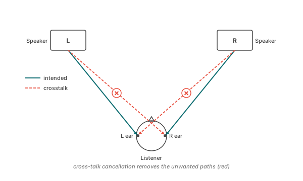
Figure 9.7. Cross-talk cancellation theory. Consider a symmetrically placed listener and two loudspeakers. The cross-talk signal paths describe how the left speaker will be heard at the right ear by way of path Rct, and the right speaker at the left ear via path Lct. The direct signals will have an overall time delay t and the cross-talk signals will have an overall time delay t + t’. Cross-talk cancellation techniques eliminate the Lct path by mixing a 180° phase-inverted and t’-delayed version of the Lct signal into the L signal, and similarly for Rct.

Auralization

Auralization involves the combination of room modeling programs and 3D sound-processing methods to simulate the reverberant characteristics of a real or modeled room acoustically. “Auralization is the process of rendering audible, by physical or mathematical modeling, the sound field of a source in a space, in such a way as to simulate the binaural listening experience at a given position in a modeled space” — see Kleiner, Dalenbäck, & Svensson, “Auralization — an overview,” J. Audio Eng. Soc. 41(11), 1993, pp. 861–875.

Auralization software/hardware packages advance the use of acoustical computer-aided design (CAD) software and, in particular, sound system design software packages. Acoustical consultants and their clients can listen to the effect of a modification to a room or sound system design and compare different solutions virtually.

The same head-related rendering that places a virtual source in a modeled room can also carry a source past the listener. The bonus page Sirens & FM includes a Doppler pass-by toggle: a siren crosses in front of the listener while the pitch shift is applied to the entire spectrum — both center frequency and deviation — as the physics requires, rather than to the center alone.

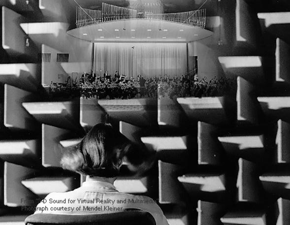
Figure 9.8. A listener in an anechoic chamber experiencing a virtual concert hall, created by applying auralization techniques.

The potential acceptance of auralization in the field of acoustical consulting is great because it represents a form of (acoustic) virtual reality that can be attained relatively inexpensively. Although computationally intensive, the power and speed of real-time filtering hardware for auralization simulation is continuously improving due to the ongoing development of improved DSP techniques, both on-board and within external devices. Compared to traditional methods using blueprints and scale models, auralization software-hardware systems allow physical and perceptual parameters of a room model to be calculated and then parametrically varied. The variation in acoustic parameters can then be verified by listening, within the limits of the accuracy of the reverberation modeling and 3D sound presentation techniques used.

Prior to the ubiquitousness of the desktop computer, the analysis of acoustical spaces mostly involved architectural blueprint drawings and/or scale models of the acoustic space to be built. Relatively unchanged is the technique of making an analogy between light rays and sound paths to determine early reflection temporal patterns, by drawing lines between a sound source, a reflective surface, and a listener location. This “geometrical approach” to eliminating noticeable echoes was born around the beginning of the twentieth century, concurrent with Wallace Sabine’s mathematical approach to determining reverberation time from an enclosure’s volume. These two developments flag the birth of modern architectural acoustics, the science of predicting and correcting the effects of an enclosure on sound quality through control of reverberation.

Figure 9.9 shows an early attempt to correct concert hall acoustics by Gustave Lyon, director of the French musical instrument manufacturer Pleyel. He stands in uniform next to an assistant inside of a sound absorbing box (called the Cage aphone). This box contains a sort of funnel at the top that can be precisely aimed at various parts of the concert hall. The hall was caused to resonate at various locations by a wood clapper device; by listening to the reverberation with the narrow audio focus made possible with the funnel, the exact location of reflecting surfaces that caused distinct echoes. Following this sort of analysis, absorptive material could be strategically placed so that the early reflections hitting these surfaces could be absorbed, and thereby attenuated by the time they reached the listener.

Figures 9.9 and 9.10 show examples of early “before” and “after” treatment of disturbing echoes in the Concert Hall of the Palais du Trocadéro (built in 1878 for the Universal Exhibition), by Gustave Lyon. Note the covering of absorptive felt in the cupola in Figure 9.10 above the organ pipes.

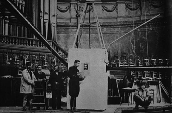
Figure 9.9. Gustave Lyon and an assistant analyzing the location of echoes in a special soundproof box (the Cage aphone); the sound funneling device for aiming towards various wall surfaces extends outwards from the left side.

Figure 9.10. Concert Hall of the Palais du Trocadéro before acoustic correction.

Figure 9.11. Concert Hall of the Palais du Trocadéro after acoustic correction. Note the absorptive material that has been placed in the cupola above the organ pipes.

While eliminating echoes was one good reason to perform an acoustic analysis of early reflections, it took decades for architectural acoustics to discover that the spatial time-intensity pattern of early reflections is also important. In particular, it is now possible to predict how the spatial incidence of reflections to a listener affects perceived quality of a room. In the early twentieth century, architectural acoustics shared roughly the same maxim as the classic Greek theater — to reflect as much sound intensity as possible towards the audience’s direction.

Figure 9.12 shows the Salle Pleyel in Paris, designed in the late 1920s by Gustave Lyon, based on his research in improving the Palais du Trocadéro hall seen in Figure 9.9. It is designed with a curving overhang over the stage, which certainly propelled reflected energy outwards, in contrast to the cupola seen previously in Figure 9.9. But note that this design does nothing to propel reflections from lateral directions towards a listener. It is now known that having early reflections arrive from side directions is preferable to reflections that arrive first from above or in front. Within certain limits, the more that early reflections are binaurally differentiated — i.e., in “stereo” — the more preferred are the acoustics. Incidentally, this is a feature imitated by some surround sound processors.

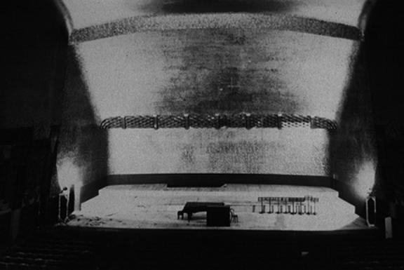
Figure 9.12. The Salle Pleyel. Note that the reflective shell behind the stage focuses early reflections forwards but not sideways.

How Auralization Systems Work

An auralization system consists of software that inputs the parameters of a room design, and outputs physical, perceptual, and simulation data. The simulation data consists of filter parameters that are either piped to a 3D audio hardware device for DSP simulation, or are computed on the host computer itself. An anechoic sound (recorded without reflections) is then input through these filters for virtual simulation of the direct and reverberant sound field. The software calculates the intensity, time delay and spatial incidence of reflected sound from source to surface to listener. Each surface, such as the walls, curtains, people, and seats in a concert hall, will have a specific filtering effect on the reflection. Early reflections are calculated individually; a statistical approach is often used to model the dense number of reflections present in late reverberation.

One begins in an acoustical CAD system by representing a particular space through a room model. This process is a type of transliteration, from an architect’s blueprint to a computer graphic. A series of planar regions must be entered to the software that represent walls, doors, floors, ceilings, and other features of the environmental context. By selecting from a menu, it is usually possible to specify one of several architectural materials for each plane, such as plaster, wood, or acoustical tiling. In reality, the frequency-dependent magnitude and phase transfer function of a surface made of a given material will vary according to the size of the surface and the angle of incidence of the waveform. In most auralization programs, the magnitude transfer function is simplified for a given angle of incidence, due to computational complexity.

Once the software has been used to specify the details of a modeled room, sound sources may be placed in the model. After the room and speaker parameters have been joined within a modeled environment, details about the listeners can then be indicated, such as their number, head-direction, and position. Prepared with a completed source-environmental context-listener model, a synthetic room impulse response can be obtained from the acoustical CAD program. A specific timing, amplitude, and direction for the direct sound and early reflections is obtained, based on the ray tracing or image model techniques described ahead. Usually, the early reflection response is calculated up to around 100–300 ms. The calculation of the late reverberation field usually requires some form of approximation due to computational complexity. A room modeling program becomes an auralization program when the room impulse response is spatialized in relationship to a virtual listener.

Figure 9.13 shows the basic process involved in a computer-based auralization system intended for headphone audition. The model also will include details about relative orientation and dispersion characteristics of the sound source, information on transfer functions of the room’s surfaces, and data specifying the listener’s location, orientation, and HRTFs.

Figure 9.13. The basic components of the signal processing used in an auralization system.

Auralization in Practice: CATT-Acoustic

CATT-Acoustic is an example of an integrated approach to the calculation of a virtual environment through the use of acoustical CAD and auralization techniques. In the following figures, the variety and complexity of analytical information used by the acoustical consultant and the architect are shown. At the end of these examples, it becomes possible to listen to — or auralize — a modeled acoustical space, from different locations.

Figure 9.14 shows a perspective view of a concert hall. The dashed blue lines intersect on the location of a modeled sound source, while the numbers refer to five seating locations to be analyzed. Each surface is modeled according to its particular frequency-dependent absorption and diffusion characteristics. Figure 9.15 shows how the software allows viewing an enclosure from different perspectives, via a GUI (graphical user interface) (this example shows the interior of a church). It is possible to navigate through and around an enclosure, in a manner similar to exploration within a virtual world.

Figure 9.14. Perspective view of a hall: the Espace des Arts (Chalon-sur-Saône, France: A. Moatti, architect and theater consultant; B. Suner, acoustical consultant).

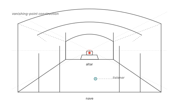
Figure 9.15. A view inside of a church, with controls for changing view perspective.

Once all of the parameters are determined for an enclosure such as shown in Figure 9.13–13, it is then possible to execute an acoustical analysis of the early reflections and dense reverberation pattern for the indicated seating positions, and derive a binaural impulse response for virtual acoustic modeling. Figure 9.16 shows the ray trace of an individual early reflection, in its path from the source to the listener.

Figure 9.17 shows a section view of the hall that can be thought of as a “spatial calculation” of the early reflections, as determined by image model ray tracing. The size of each circle corresponds to the reflection intensity, the distance corresponds to time delay, and the location corresponds to the relative angle of incidence to the listener. Figure 9.18 shows the resulting binaural impulse response; the large peaks correspond to strong reflections within the enclosure.

Figure 9.16. Ray trace of an early reflection (close-up of Figure 9.14).

Figure 9.17. Spatial calculation of the intensity of virtual images. Left: side view; right: forward view. The size of the circle is the intensity of the reflection; the distance from the hall is the time delay; and the location is relative to a listener seated in the hall.

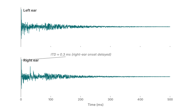
Figure 9.18. Binaural impulse response.

Auralization Listening Examples

Figure 9.19, an overhead view of the hall shown in Figure 9.14, allows one to auralize the environment as if seated at three different positions (labeled .01, .02, and .05). By clicking or tapping on the following items, the increase in the complexity of the acoustical simulation becomes audible. The number of early reflections modeled ranges between:

• None — direct sound only (D)
• First–fifth order (1–5)
• A complete simulation with late reverberation (E+R)

The examples demonstrate how a sound field consists of an increasingly complex set of reflections, and how each can have an important influence on the resulting reverberation. However, note that both late reverberation and early reflections are important to forming a recognizable virtual acoustic image.

First, listen to the original anechoic sound: click or tap here

Figure 9.19. Overhead plan of hall shown in Figure 9.14. Use the buttons below to hear direct sound, increasing orders of early reflections, and complete simulation for each seating position.

Head Movement and Virtual Acoustics

It was pointed out earlier in this chapter that head movement can contribute substantially to the realism of a virtual acoustic simulation. The Binaural Spatializer demo above demonstrates this directly: rotate the listener’s head with the slider and hear the source apparent direction shift in response, via Web Audio’s HRTF listener-orientation API. (When the original Sonic content was authored, this was “beyond the technology of a static web page” — modern browsers have since closed that gap.) Recipes for exploring head rotation: place the source directly behind and sweep head rotation ±30° to resolve the front/back ambiguity; or fix the source at 90° right and rotate the head to +90° so the source aligns with the nose axis.

Two prerecorded comparisons follow, using someone else’s head movement synthesized with CATT-Acoustic and the “HeadScape” software / “Huron” hardware system from Lake DSP:

Bonus: The Shepard Tone Illusion

One of the most striking auditory illusions related to pitch and spatial perception is the Shepard tone — a sound that appears to ascend (or descend) in pitch endlessly, without ever actually getting higher (or lower). Named after cognitive scientist Roger Shepard, this illusion is created by layering multiple sine waves spaced an octave apart, with their amplitudes shaped by a Gaussian envelope so that tones fade in at the bottom and fade out at the top (or vice versa). The result is a sonic equivalent of the endlessly ascending staircase optical illusion by M.C. Escher. Shepard tones are widely used in film sound design to build tension and create a sense of perpetual motion.

Try it → the full interactive Shepard Tone explorer lives on its own page: Shepard Tones & the Endless Staircase. It includes a 12-step Escherian Penrose staircase that can be walked with the keyboard or by clicking or tapping, a linear-piano + radial keyboard pair, glissando across both, chromatic / diatonic modes, multi-voice synth (true gapless sustain), and several preset envelopes — far more than would fit in a chapter sidebar.

Bonus: ASMR Sound Walk

The same HRTF panning that powers the spatializer above also produces the close-mic’d, “coming-from-right-beside-the-ear” quality that defines most ASMR content (Autonomous Sensory Meridian Response). The illusion of intimate proximity is a binaural phenomenon, not an acoustic one: the same brainstem cross-correlator that placed clicks or taps behind the listener in the spatializer also lets a synthesized tap circle one ear at conversational distance and feel like it’s only inches away.