Digitization and Editing
How analog sound becomes digital data through sampling and quantization, and the essential editing workflow: recording, cropping, normalization, trimming, and file management.
Sampling and Quantization
Digital sampling is the term used in digital audio technology for the process of converting a continuously varying electrical voltage into a sequence of numbers for computer storage. An analog-digital (A-D) converter samples the relative voltage of the analog signal at equally-spaced moments of time, and then stores each value sequentially. The number of times the analog signal is evaluated over one second is termed the sampling rate, which is measured in terms of frequency. The audio sampling rates most commonly encountered in digital audio are 44,100, 48,000, and 96,000 Hz; meaning that the analog signal is evaluated that many times each second. The process of assigning a digital numerical value proportional to the voltage level at each sampled moment is termed quantization; typically, 16- or 24-bit digital words are used to represent each sampled voltage level.
A good analogy for the difference between an analog signal and digital sampling is the comparison between a traditional clock with hour, minute, and second hands, and a digital clock with a numeric display. On a traditional clock, time is represented continuously by the motion of the second hand. This is equivalent to the continuous analog voltage variation that is found at the output of a microphone or a loudspeaker. Contrasting this, a digital clock display changes in increments of the smallest value of time shown (usually every second). The display doesn’t indicate anything “between the cracks;” the passage of time is displayed only in increments of the sampling rate of once a second.
To understand how sampling and quantization work together, consider the analogy of a black and white movie camera. This will sample an “analog” visual scene at a rate of 24 frames a second; nothing that occurs in the time interval in-between the frames will be captured. Furthermore, within each sampled frame of film, the color spectrum is quantized into a particular grayscale value from black to white.
Another way of understanding quantization is in terms of a questionnaire used in a survey, for instance to determine how a respondent feels about a political candidate or snack food. Complex “analog responses” in the form of a qualitative opinion are seldom solicited. Instead, a discrete set of quantized responses is given, from which to choose. For instance, a “true-false” or “yes-no” questionnaire is equivalent to a quantization granularity of 2. The possibility of “maybe” is lost because the resolution is too coarse with such a “two-alternative forced choice” paradigm.
Now, let’s apply these concepts to audio. Recall from Figure 5.1 that the overall process involves analog-digital conversion for storage and subsequent digital-analog conversion for playback. The implication is that the signal during playback will have only as much detail during D-A conversion as the amount of detail used in recording via A-D conversion. Just as color can never be extracted from a black and white film (it can only be added artificially), no frequency or intensity information can be recovered from a recorded audio signal that the initial A-D conversion did not capture.
In Figure 6.1, a 100 Hz analog sine wave is shown in red; the analog x and y axis values are also in red, at the top and at the right of the figure. The equivalent digital values are shown in blue x and y axis values at the bottom and the left of the figure. One period of a 100 Hz waveform takes 0.01 seconds to complete; the variation in intensity of the analog voltage is shown as ranging from ±1. The blue lines represent equally-incremented sequential values of the analog waveform, resulting from sampling the waveform at a rate of 2000 Hz. Twenty “snapshots” (sample values) of the analog signal’s intensity are measured during .01 second, which are (more than) sufficient for the digital audio system to accurately reconstruct the waveform upon subsequent D-A conversion.
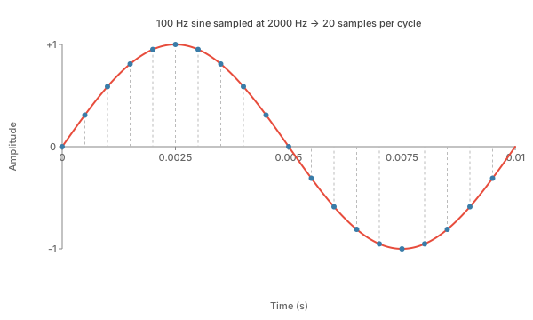
Figure 6.1. An analog waveform (red) and its digital representation (blue).
In Figure 6.1, the signal is quantized into the range of numbers available from a signed-integer, 16-bit representation. This means we can represent the upper peak voltage value of the analog sine wave at 1.0 volts with the largest signed integer, 32767, and the lower extreme with –32767. Variations within the voltage range ±1 are stored at proportional digital values in the range ±32767. For instance, if an analog voltage amplitude at a single moment in time was 0.25, then the nearest integer digital value would be 8192 (0.25 × 32767 = 8191.75, 8192 when rounded up). Figure 6.2 below shows the stream of numbers that result. Note the similarity between the symmetrical pattern of the numerical representation and the graphical representation of the waveform.
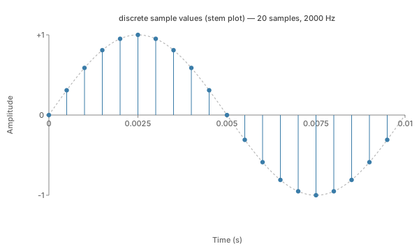
Figure 6.2. Sampled version of the sine wave shown in Figure 6.1. At a sampling rate of 2,000 Hz, 20 samples per cycle of a 100-Hz sine wave would be obtained, corresponding to the blue values on the y axis of Figure 6.1.
Figure 6.3: Sampling Rate & Bit-Depth Quantizer
Hear the Nyquist theorem and quantization noise directly, not just in equations. Pick a source and reduce its sample rate to hear aliasing (folded high-frequency partials reappearing low in the spectrum); reduce its bit depth to hear the hiss / crunch / fuzz of low-resolution quantization. Try the “Tape” or “Telephone” presets for canonical examples.
Implications of Different Sampling Rates
In Figure 6.1, twenty samples were used to represent a 100 Hz sine wave at a 2000 Hz sampling rate. Equivalent sampling would yield ten samples of a 200 Hz sine wave, five of a 400 Hz sine wave, etc. Theoretically, A-D and D-A converters need a minimum of two samples to represent a waveform; this is known as the Nyquist theorem, which states that the highest frequency that can be represented by a digital system can be no higher than half the sampling rate. Frequencies above the Nyquist frequency — that is, above half the sampling rate — are subject to digital foldover, which is a type of harmonic distortion. Digital foldover is eliminated in a digital system by using low-pass filtering prior to sampling, an analog circuit that removes energy above the Nyquist frequency before the signal reaches the converter.
What this all means is that when sampling a sound for a digital recording, only frequencies up to half the sampling rate are captured. Recall that the range of human hearing is from 20 Hz–20 kHz. A “low” quality sample rate of 11 kHz will only yield frequencies on playback up to around 5500 Hz. In fact, analog filters have certain imperfections in how accurately they can cut sound at a particular frequency, so that the highest frequency available will be slightly less than half the sampling rate. A frequency range with an upper boundary of 5500 Hz will yield intelligible speech but makes everything sound like it’s being played through a telephone loudspeaker. The “medium” and “high” quality sampling rates of 22 kHz and 44.1 kHz (the standard sampling rate for CD-quality audio) on the other hand cover most of the energy heard in everyday sounds. In fact the 22 kHz sample rate is useful for most purposes because only the highest partials of a complex sound have energy above 11 kHz, and these are relatively weak. But for critical listening applications, a sampling rate of at least 44.1 kHz is essential. Modern professional audio commonly uses 48 kHz or 96 kHz for even greater fidelity.
The following examples give a quick hearing of the effect of different sampling rates:
| Speech | Pink Noise |
|---|---|
Notice that the effect is much more dramatic for the pink noise than for the speech. Remember that pink noise has an equal amount of energy within each octave, while speech contains most of its energy below 5 kHz.
Implications of 8- and 16-bit Quantization
The process of converting from an analog to a digital signal system involves quantization, the assignment of one of a set of digital values to represent a range of analog voltage levels. The choice of quantization bit depth is manifested in how many possible values are available within the digital system to represent the momentary intensity of a sampled analog signal. It’s obvious that a digital system uses numbers, but perhaps less obvious is the fact that the number of bits used to represent these numbers implies the range of numerical values that can be used by a digital system. With sampling rate, the highest frequency that can be captured is related to the “horizontal granularity” of how often samples are taken. The “vertical granularity” on the other hand relates to the quantization of the signal according to the number of bits.
A bit is a binary integer that can have the value of 0 or 1; the range of numerical values is 2 to the power of the number of bits. Now consider a hypothetical 2-bit A-D converter, which would have a quantization range of (22 =) 4 values. Each sampled analog voltage value is assigned one of the 4 different combinations possible with two bits: 00, 01, 10, 11. If we have a voltage range of ±1 as in Figure 6.1, the following relationships between the voltages and their quantized values shown in Figure 6.4 would apply:
| Bit no. | Bit assignment | Voltage lower limit | Voltage upper limit |
|---|---|---|---|
| 1 | 00 | –1.0 | –0.5 |
| 2 | 01 | –0.5 | +0.0 |
| 3 | 10 | +0.0 | +0.5 |
| 4 | 11 | +0.5 | +1.0 |
Figure 6.4. 2-bit Quantization.
Such a 2-bit system is impractical for audio because most of the variation within the lower and upper analog voltage limits would be lost through quantization. Just as under-sampling a sound with a low sample rate causes high frequencies to be lost, with correspondingly degraded sonic results, under-quantization will cause a sampled waveform to differ radically from the original waveform of the input, due to loss of “vertical granularity.” A good analogy is the way that a picture progressively loses its original color as a function of the number of bits used to quantize the image on a monitor (see Figure 6.5).
With an 8-bit system, there are (28 =) 256 possible values; see Figure 6.6 below. Note that the range of each voltage is smaller since there are a larger range of numbers that can be assigned. This is adequate for representing some sounds, such as speech or electronic sounds in a game, but no more than adequate; 16-bit quantization is vastly superior and is the standard for CD-quality sound. Modern professional audio typically uses 24-bit quantization for even greater dynamic range.
Two things are worth adding to that ladder, because both are routinely misread. The first is 32-bit float, now common as a recording and processing format. It is not a converter specification: no analogue-to-digital converter resolves anything like the range the format can hold, and the physics of a microphone and its preamplifier stop long before that. What the format buys is headroom and safety inside the computer — intermediate results can exceed full scale and come back without clipping, and a take recorded far too hot can be brought down afterwards intact. The converter in front of it is still a 24-bit part, and its noise floor still sets what was actually captured.
The second is what happens at the band edge. The Nyquist argument assumes everything above half the sampling rate has been removed before sampling, and a filter that passed everything below and nothing above would have to be infinitely steep, which is not a thing that exists. Converters therefore oversample: they run the conversion at several times the nominal rate, where the filter has octaves rather than a hairline in which to do its work, then filter digitally and reduce to the output rate. The gentle analogue filter and the steep digital one together do what neither could alone. This is why sampling-rate diagrams showing a vertical wall at Nyquist are a schematic convenience rather than a picture of a real converter.
Figure 6.5: Bit-Depth Quantization of a Visual Image
A direct visual analog of audio bit-depth quantization. Drag the bit-depth slider to set the number of distinct levels per color channel; drag the round handle on the vertical seam to wipe the seam across the image. Pixels to the left of the seam show the full 8-bit-per-channel original; pixels to the right show the reduced-depth version. As the depth drops below about 4 bits/channel, smooth gradients break into visible bands — the visual counterpart of the quantization noise heard in low-bit-depth audio.
Figure 6.5. Bit-depth quantization of a visual image. The left half stays at 8 bits/channel; the right half drops to the chosen bit depth. Posterization in the visual domain is the direct counterpart of quantization noise in the audio domain.
| Bit no. | Bit assignment | Voltage lower limit | Voltage upper limit |
|---|---|---|---|
| 1 | 00000000 | –1.0 | –0.992 |
| 2 | 00000001 | –0.992 | –0.984 |
| ⁚ | |||
| 255 | 11111110 | 0.984 | 0.992 |
| 256 | 11111111 | +0.992 | +1.0 |
Figure 6.6. 8-bit quantization.
8-bit audio survives now only where storage or bandwidth is unusually tight. In a 16-bit system, there are (216 =) 65,536 possible values; compared to the 256 possible values in an 8-bit system, the sound quality of 16-bit sound is a dramatic improvement. A jump from 8 to 16 bits can also be heard in terms of the improvement in the signal-quantization noise ratio (SQNR). This refers to the dynamic range of the signal that can be captured by the digital system, relative to the digital noise floor (all bits at 0). An 8-bit system has a dynamic range of 20 log10(28) ≅ 48 dB, while a 16-bit system has 20 log10(216) ≅ 96 dB. Recall from Figure 2.4 that the dynamic range of the environment is at least 120 dB SPL, and that better microphones are within 10 to 20 dB of this range. Although the dynamic range of 16-bit quantization is sufficient for capturing most recorded material, professional systems commonly use 24-bit quantization, whose ideal range of about 144 dB is a property of the word length rather than of any converter: the analog noise floor ahead of it gives out first, and a converter’s effective number of bits is what says where. Low sample rates and short words are still chosen deliberately — for transmission bandwidth, for computation, for latency, or for the limits of a small device — rather than to save disk space.
Figure 6.7 below summarizes the storage requirement for one second of sampled sound, for common configurations of sampling rates and quantization rates. For a stereo (2 channel) sound, the storage requirements double.
| No. of bits | Sampling rate | Storage requirement | Sound example |
|---|---|---|---|
| 8 | 11.025 kHz | 11 kbytes | |
| 8 | 22.05 kHz | 22 kbytes | |
| 16 | 22.05 kHz | 44 kbytes | |
| 16 | 44.1 kHz | 87 kbytes |
Figure 6.7. Disk storage requirements for one second of linear (uncompressed) audio.
It is possible to reduce the storage requirements via sound file compression. Most compression schemes involve a loss of some information between the original sound file and its compressed version. A sound file can also be “down-sampled” or “down-quantized” to a lower rate with some software packages. These topics are covered in Chapter 7.
The trade-off between storage and sound quality needs to be considered for any large project; sound files have a way of taking over most of the space available. Note that a minute of stereo “CD quality” sound (at 16-bit quantization, 44.1 kHz sample rate) requires about 10.1 megabytes of storage as uncompressed PCM — the form a recording is worked on in. A compressed delivery format holds the same minute in a fraction of that, which is why a finished file and a working file are such different sizes. Some software also keeps a backup copy of the sound file being edited so that edits can be undone, thereby occupying additional storage space.
The Software Recording Environment
To record sound onto a computer disk, sound editing software as well as an audio interface are needed. The software provides facilities for recording, editing, and formatting sound files, and sometimes digital signal processing for effects. A generic software system would include recording and playback controls and a time-intensity waveform display such as those presented in this site.
Figure 6.8 shows a typical display; the x axis indicates time and the y axis indicates intensity of the waveform. The software should allow dragging the mouse over a section of the waveform to cut or copy it for pasting at another point in the same waveform or into another window. The waveform display can usually be zoomed in or out to several levels. Zooming in (sometimes to where each individual sample value is visible) is done when it is necessary to examine the waveform with sufficient detail for critical editing. Zooming out to a larger overview of a sound is necessary for making initial crops of the waveform and arranging sections of sound (see Figure 6.9).
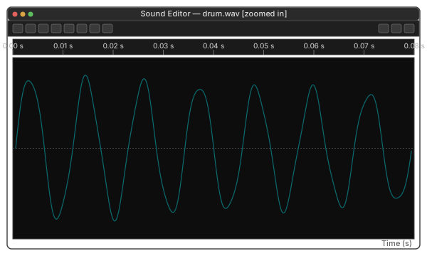
Figure 6.8. A sine wave, viewed by zooming in on the sound file waveform display.
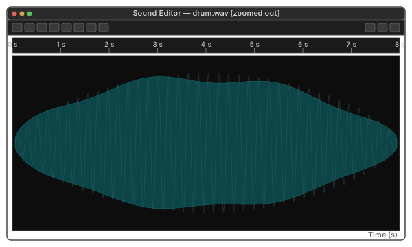
Figure 6.9. The same sine wave as in Figure 6.8, zoomed out.
It is possible to get into a rhythm of capturing sound files from a sound source such as a streaming service, audio player, or a sampler by going repeatedly through the following steps:
- Opening and formatting a sound file;
- Recording (sampling, capturing) and checking levels;
- Cropping;
- Normalization;
- Trimming;
- Mixing among tracks; and then
- Naming and saving the sound file.
Opening and Formatting the Sound File
To begin recording, the first step is to open a new sound file and set its format. Usually there is a selectable menu feature for indicating the quantization level and sampling rate to be used. Advance planning should ensure that there will be adequate disk storage space for the waveforms that will be recorded. Practically speaking, longer sounds are edited into smaller segments to make playback and editing easier. Part of the art of composition involves the ability to form the time sequence of sounds in a successful manner. Although the final production involves organization on a larger time scale, it is better to record sound files as smaller segments that are then combined at a later time (for instance, groups of sentences rather than an entire narrative).
Recording
Most audio interfaces have either RCA jacks (usually white “left” and red “right,” as in Figure 6.10), a stereo miniature jack (seen previously in Figure 5.9), or more commonly today, XLR and 1/4” TRS combination inputs for connecting the output of the sound source to the input of the A-D converter. After making a good connection, the first task is to determine if the input level is too low (which results in excessive noise) or too high (which results in distortion). Usually, the sound editing software will have the equivalent of a VU (voltage units) meter that allows monitoring the input level (see Figure 6.11).
The VU meter indicates the dB RMS value relative to the headroom of the A-D converter. A value of 0 dB VU is the “hottest” signal the hardware can handle, with values below this expressed in negative dB values. In some cases there is a built-in software attenuation control as well, but often the output from the sound source (perhaps via an analog mixer or microphone preamplifier) will need to be adjusted. See Chapter 2 for additional details regarding relative dB VU levels.
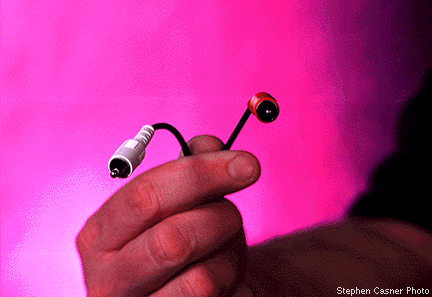
Figure 6.10. RCA pair connectors.
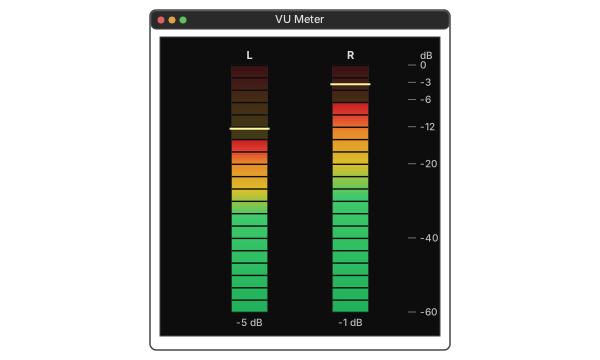
Figure 6.11. Software VU meter.
Live VU Meter
Software meter responding to live audio. Pick a source, drive the pre-meter gain into the red, and compare three classic ballistic conventions: VU (slow RMS integration — the standard described above), PPM (faster peak-program meter), and instantaneous peak. The peak-hold marker (thin vertical line) holds the highest recent reading; the CLIP LED lights any time the signal touches 0 dB.
With analog sources, mixing engineers may be used to pushing levels “into the red,” up to +3 dB or even higher, possible because analog tape has a certain amount of headroom. Headroom is an intensity range above a certain maximum value reserved for sound peaks (transient amplitude values). The theory is that most of the signal will be within the RMS intensity range, at intensities up to a nominal level, while the peak of the amplitude envelope of a sound or group of sounds will go beyond this. With a digital recording, there is no headroom above 0 dB VU. This necessitates setting the nominal level to around –12, or even –20 dB VU. The relationship between RMS values and peak values is visible if the input VU meter has a peak indicator, which lights up each time the upper limit of the headroom is exceeded.
Once a test recording has been made, the waveform can be checked for whether or not there is any signal or if the peak value has been exceeded. It will be obvious when some sort of waveform is present. If nothing seems visible, and the connections have been checked, try zooming in on the y axis on a portion of the waveform where the sound source was silent, or amplifying a portion of the silent section. Most systems will have some residual noise present if the microphone or other device is actually hooked up (see Figure 6.13).
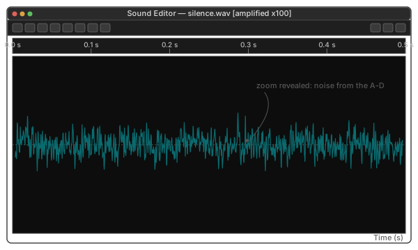
Figure 6.13. Zooming in by amplifying a selected section of a waveform, to determine if system noise is reaching the input. This illustration indicates that some sort of noise is reaching the A-D from an external source. If amplification had resulted in no change, then no signal is reaching the A-D.
Some software will search and display the sound file’s peak value and the time when it occurred. Otherwise search the sound file by zooming in and then scrolling through it, looking for the maximum or minimum intensity values. No sample should reach beyond 100 % intensity (the quantized values of ±32767); if it does, then clipping distortion has likely occurred. Figure 6.14 shows the characteristic “flat top” of a clipped waveform when viewed zoomed in; at right is the unclipped version of the waveform.
Waveform clipping was introduced previously in Chapter 2 (see Figure 2.5) in the discussion of dynamic range. The dynamic range of the recording system must be accommodated via proper setting of the input level, so that the dynamic range of the input signal —including its peak values— do not exceed the range of the recording device. As shown previously in Chapter 2 (Figure 2.4), the challenge of recording and playback is to accommodate mismatched dynamic ranges from one medium to another. Practically speaking, an analog or digital compressor can be used to narrow the dynamic range of a sound source; compression is discussed in detail in Chapter 7.
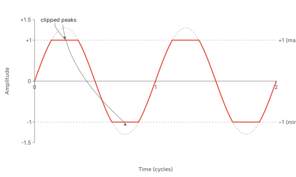
Figure 6.14. The flat top of a peak signal, indicative of a clipped waveform with a non-normalized sound file.
Figure 6.15: Live Clipping & Headroom
Drive any source past 0 dBFS and watch the waveform develop the flat top of Figure 6.14. The before (gray) and after (red) waveforms overlay so the clipping is visible. Use it to hear how a soft sine becomes a buzzy square as the gain is pushed — that’s the textbook mechanism for harmonic distortion.
Cropping
Cropping the waveform involves isolating the usable portion of the recording. There should be no “dead space” at the beginning or ending of the sound file. First, zoom out and mouse over what visually appears to be the usable portion of the waveform, and then listen to the result (see Figure 6.16). Once the region has been isolated, the idea is to not cut off any of the first sound’s initial attack, nor any of the last sound’s decay.
for an example of a speech sound file that has been cropped too narrowly, trimming off some of the attack.
for an example of a sound file that has been cropped just at the start of the speech.
for an example of a sound file that has been cropped so that the sound of inhaling before the word is preserved. This may or may not be desirable for the final recording.
The “fine tuning” of the beginning and ending of the moused-over section can be accomplished by zooming in, and then adjusting the selection slightly, listening while doing so. Some software packages have a trim or crop function that deletes any part of the sound file that hasn’t been selected. Otherwise, two separate steps are needed to delete the dead spaces; mousing over those sections, and then using the delete key (or its equivalent).
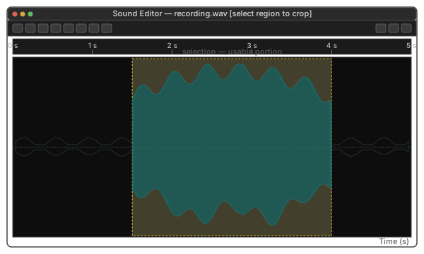
Figure 6.16. Cropping the waveform by isolating the usable portion of the recording.
Normalization
Normalization means that the intensity of a sound file is multiplied so that its peak value equals 100 % of the intensity. This results in an overall gain to the sound file, so that the recorded signal fills the entire quantization range. The software uses a two-step process. First, the entire sound file is searched for its peak value; second, whatever coefficient is necessary for scaling the peak value to maximum intensity is applied to the entire waveform.
Note that using normalization on a set of sound files doesn’t mean that they will have the same loudness. This is because the peak intensity values of two sound files may be the same, but their RMS values could be widely different. If a sound file has an intermittent transient at peak intensity (e.g., caused by momentarily shorting of the input connection) the normalization will be based on this spurious value. Normalization is also not a substitute for getting as much level in the initial recording as possible. The process amplifies all of the signal and the noise in the sound file.
to listen to a normalized recording of a sound file that was made with a relatively “hot” input level; and to listen to a normalized recording of a sound file that was made with an inadequate input level. Note that this second example contains much more noise in the recording.
In many cases, it is best to normalize at a later stage of production. For instance, if there are 10 narration sound files to be adjusted so that they are about equally loud, it’s sometimes better to: 1) balance out non-normalized files for equal loudness by ear and a software gain adjustment; 2) find the file with the highest peak value and normalize that file only; 3) determine the amount of gain used to normalize that file; and then 4) apply that gain level to all of the rest of the files.
Fine Trim (Splicing)
Sometimes editing within a cropped sound file is necessary, between words, sounds or even syllables or individual notes. This can be referred to as “fine trim,” and in many cases can be very challenging. Previous to digital audio, this was accomplished by splicing, i.e. cutting analog audio tape into smaller sections and then re-assembling the parts. It is a little-known fact that many studio recordings of classical music are made up of multiple performances; the best performances of each musical section are spliced together to create a performance different (and often superior) to what the artist can achieve in live performance. These can be as broad as entire movements, or as detailed as individual notes; it is not uncommon for a recording of a single piano sonata to be made up of 40 or more splices. The practice has become easier with the advent of digital technology.
Figure 6.17 shows a waveform display of the spoken word “Lovesickness.” to listen to the sound. By editing within the middle of the word, we can transform the sound into the word “sickness.”
What we will attempt to do is to edit between the point of the “v” sound in love and the “s” sound that begins “sickness.” The first step will be to mouse over various sections of the waveform and then play them back. In Figure 6.17, we have written the approximate location of the different sounds. Note the pattern of the waveform seems to change with the particular vowel or consonant that is being said. These individual speech sounds are referred to as phonemes. For instance, the first distinctive change occurs in the transition from “Lo” (sounds like “Luh”) to “ve” (which sounds like “vi” or “vuh”, depending on the pronunciation).
Now say the word “love” slowly and observe what happens with the mouth and tongue while saying the word. The “l” part involves touching the tongue to the back of the teeth, and the “o” occurs in the release ( to listen to this). This particular phoneme is quite distinct from the “v” part of the sound, where the upper teeth are brought into contact with the bottom lip ( to listen to this). Compare this to what happens on saying the word “lumber” slowly; the “lum” part is the same “lu” sound but the lips are brought together rather than making contact with the teeth. Now look again at the waveform in Figure 6.18, where we have zoomed in on the transition point. It looks similar in the Lu and V sections. This is because in the word “lovesick” less time is spent on the v sound, instead proceeding directly onto the “ss” sound. But it is very obvious where the “s” sound begins since it is more noise-like.
This is obviously the region at which to make our splice. But to determine an exact location, the best technique is to find the zero crossing point of the waveform. Figure 6.19 illustrates this in detail. Splicing at a zero crossing point avoids clicks or taps, and allows merger with the beginning of another word whose start point has been cut at a zero crossing point.
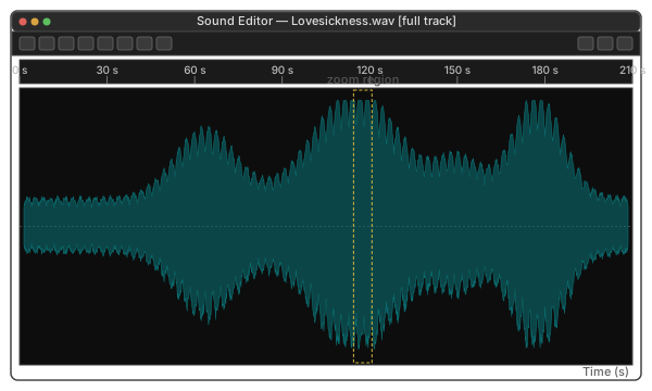
Figure 6.17. The waveform “Lovesickness”, zoomed out.
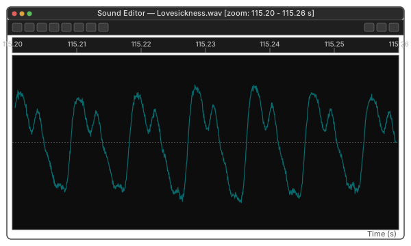
Figure 6.18. The waveform “Lovesickness”, zoomed in.
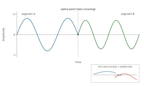
Figure 6.19. Editing waveforms at the zero crossing point avoids clicks or taps and allows the end of one waveform to be more easily spliced to the start of another.
Naming and Saving the Sound file; Formats
Once the previous steps are completed, the sound file can be named and saved for later processing or combination with other sound files. At this point the sound file can be saved in any of a variety of different formats. These formats have to do usually with how the sound file is stored, and with the sound file information header, a section of the sound file that contains metainformation about the sampling rate, quantization, etc., instead of pure waveform data. The most common sound file storage formats are WAV (widely used across platforms), AIFF (common on macOS), and compressed formats like MP3, AAC, FLAC, and OGG. Most modern DAWs and sound editors can read and write all popular formats. Lossless formats (WAV, AIFF, FLAC) preserve full quality, while lossy formats (MP3, AAC, OGG) achieve smaller file sizes at the cost of some audio fidelity.
Every computer hardware and software system will have peculiarities unique to that system, and most provide adequate information within their documentation. Practice editing and recording before jumping into a major project, using both eyes and ears, so as to make a connection between the visual display and the actual sound.