Utilities and Effects: Digital Signal Processing
From sample-rate conversion and compression to filtering, reverberation, and phase vocoding — the creative and practical tools of DSP.
Introduction
Changing the character of an input signal in the digital domain has been greatly facilitated by the development of DSP chips, particularly since they can imitate the behavior of most analog sound processing devices, such as mixers, delays, filters and analyzers. Other advantages made possible by DSP include smaller hardware size, greater control over noise floors, and ease of reconfiguration — different software specifications can be written to the signal processor, rather than re-soldering hardware components. Many DSP functions are performed by outboard (external) units. In 1996 these commonly offered better converters and more immediate control than their software equivalents, and the expectation then was that software would catch up as processing power grew. It did: the advantage has since largely reversed, and what recommends dedicated hardware today is the physical control surface and processing that does not compete with a general-purpose computer for time, rather than the quality of the arithmetic.
Digital signal processing in the context of sound software has two basic functions. The first are utility functions that have less to do with creativity than with “housekeeping” chores, similar to the normalization function discussed in Chapter 6. For instance, we might need to change the sampling rate of a sound for compatibility with another medium, or analyze the size of the file to save disc space. In the first section below, we discuss:
- Sample rate & quantization conversion
- FFT displays of spectrum
- Sound file compression
- Mixing
The second basic function of DSP is to create special effects that do anything from slightly alter to completely transform the character of a sound source. These are termed DSP sound modification functions. This application of DSP is a critical part of the creative process of sound composition. In the second section below, we discuss:
- Time delay
- Filtering
- Reverberation
- Companding
- Phase vocoding and pitch shift
Utility Functions
Sample Rate & Quantization Conversion
Sample rate conversion is a fairly straightforward, usually one-time process of changing the stored sampling rate of a sound file; either upwards (up-sampling) or downwards (down-sampling). The interaction with the software usually requires no more from the user than typing in or selecting a desired sampling rate. Many types of sound editing and processing software offer sample rate conversion routines, but the sound quality can be variable (usually as a trade-off for computational efficiency). Up-sampling and down-sampling are sometimes necessary for creating compatibility between different software or hardware mediums; down-sampling is also performed in order to conserve disc space.
In Chapter 6 presented the differences between a sound originally sampled at 44.1 kHz, and then subsequently down-sampled to 22.05 and 11.025 kHz. A sound with no noticeable energy in frequencies above half the sampling rate (the Nyquist rate) can usually be down-sampled to a lower sampling frequency without noticeable audio degradation. However, D-A converters that are part of audio interfaces are usually optimized around only a few sampling rates.
In a similar vein, Figure 6.6 showed the effect of down-quantizing a sound file from 16 to 8 bits. While a 50 % reduction in sound file size results, the dynamic range is compressed from 96 dB to 48 dB. What actually changes is the size of the quantization step. Each sample must be rounded to the nearest representable level, and with 8 bits those levels are 256 times coarser than with 16, so the rounding error — the quantization error — is correspondingly larger. Nothing is cut away at a threshold: quiet passages are not deleted, they are rendered with fewer distinct levels, and the error that results is heard as a noise floor, and on very quiet material as a gritty distortion correlated with the signal. Dither, a small amount of noise added before quantizing, trades that correlated distortion for a steady, benign hiss and is why well-made 8-bit transfers sound cleaner than arithmetic alone would suggest. Note also that the digital maximum here is 0 dBFS — decibels relative to full scale, the largest representable sample value — which is not the same reference as 0 dB VU on an analog meter; how the two are aligned is a studio operating convention rather than a fixed equivalence.
Sound file Compression
Audio compression is different than sound file compression. Audio compression refers to limiting the level of a waveform to a certain range, as part of compression-expansion (compander) processing, and is described later in this chapter. Sound file compression on the other hand refers to methods to reduce sound file size; both an encoder (“compressor”) and a decoder (“decompressor”) are necessary to create an audible waveform.
There are a number of available sound file compression schemes that all function to reduce the disc storage required by a sound file. These include MPEG layer I and II (Motion Picture Experts Group), MACE (Macintosh Audio Compression and Expansion), and ADPCM (Adaptive Delta Pulse Code Modulation). Modern formats such as MP3 (MPEG layer III), AAC, Ogg Vorbis, and FLAC are now widely used as well. These techniques usually involve a complex scheme for either eliminating data redundancy, or for eliminating data that is perceptually “transparent” (its absence should pass unnoticed). Some schemes are designed for real-time processing, while others are slower but of higher quality. Unfortunately, most compression schemes involve a “lossy” process (hence, the term lossy compression), meaning simply that some information will be lost upon compression that cannot be subsequently retrieved. Whether or not this matters is best determined by listening.
Below in Figure 7.1 are some examples of a cymbal crash that has been compressed using various methods. Listen to the noise levels, the manner in which the high frequencies die out, and the quality of the attack on the cymbal by the beater. Compare the different compression schemes aurally versus what percentage of disc storage space is saved. If storage is not an issue, compression should be avoided; it’s expensive for processing and obviously can introduce artifacts. But in many cases, especially multichannel formats, it opens up many possibilities for audio that might not otherwise exist.
| Scheme | File size | Reduction | Listen |
|---|---|---|---|
| Uncompressed, 16-bit | 120 kbytes | 100 % | |
| MPEG layer I | 72 kbytes | 60 % | |
| ADPCM 2:1 | 64 kbytes | 53 % | |
| MPEG layer II | 60 kbytes | 50 % | |
| Uncompressed, 8-bit | 60 kbytes | 60 % | |
| ADPCM 4:1 | 40 kbytes | 33 % | |
| MACE 3:1 (8-bit) | 24 kbytes | 20 % | |
| MACE 6:1 (8-bit) | 16 kbytes | 13 % |
Figure 7.1. Table of the storage and auditory effects of various compression schemes on a cymbal crash sound file. The original file is at top: uncompressed; 16-bit; 22050 sampling rate.
In practice, compression schemes must be compared on a case-by-case basis for a particular project; a particular compression method might work with one type of sound but not another.
Mixing
Mixing technically involves the summation of individually-recorded digital audio channels to a fewer number of channels. We previously introduced a diagram of a typical analog mixer (see Figure 5.14). The audio mixers that are provided with software sound editing packages are similar, except that sound files rather than live inputs are “mixed down,” typically to 1 or 2 tracks (monaural or stereo). This can be either individual sound files, or the individual tracks within a sound file.
The most obvious reason to adjust gain of individual tracks is to mix the relative levels of sound sources to a desired combination, like the level of speech against background music. But another reason has to do with the fact that the addition of multiple tracks can easily cause distortion. For instance, consider mixing two normalized amplitude sound files to one sound file; the total level would be 200 % of capacity. On analog and some software mixers, the signal gain is scaled using fader controls for each input (see Figure 7.2), while some software mixers have the user type in a percentage gain scale within an “amplitude” function. Software gain adjustments must be made to avoid clipping in the output file; some software will automatically perform this function as an option.
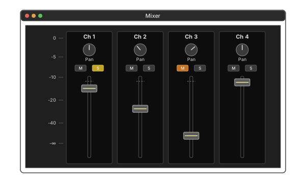
Figure 7.2. An example of software faders from a digital audio workstation.
Figure 7.3 shows a schematic version of software mixing. Two sound files, one with one track and the other with two tracks, are summed to track one of an output (destination) sound file. To avoid clipping, each sound file is gain scaled by a value of 0.5 (—6 dB on the mixer fader seen by the user). A pan (or output assignment) control is usually present, allowing mixing relative left and right levels to a stereo file. Note that in the specific example shown in Figure 7.3 we could have mixed everything to a monaural file, since the pan control is 100 % to the left. Panning allows, for instance, mixing the monaural track on sound file 1 to both channels of the destination file equally, while simultaneously mixing a stereo soundtrack on sound file 2 by copying tracks 1 and 2 to the same tracks on the destination sound file. This is common procedure with a monaural narration track against a stereo music track.
Sometimes mixing can be performed in order to form a new type of sound source. In the following example, two sounds with different amplitude envelopes are mixed. The bell () has a quickly decaying amplitude envelope with an immediate attack, while the modulated sound () has a slow attack and variable envelope. Combined, they form a completely different sound (). This idea is frequently used as a technique in music composition for acoustic instruments within a traditional orchestra.
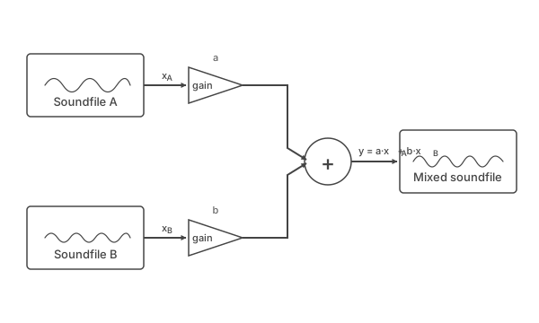
Figure 7.3. Schematic of software mixing of two sound files (three tracks) to one sound file (with two tracks).
Spectral Analysis
We can look at the harmonic content of a sound source over a single period in time by performing a Fast Fourier Transform (FFT) analysis on the waveform. The ultimate goal is to obtain a spectral analysis of a sound source, in terms of a two-dimensional frequency-versus-dB magnitude plot, or a three-dimensional plot that indicates the evolution of harmonics over time within a waveform. This is useful for determining optimal frequencies for spectral modification, or for analysis.
The Fourier transform works for sound analysis by mathematically decomposing a complex waveform into a series of sine waves whose intensities and phases can then be determined. Usually, we are more interested in the relative intensities of each of the frequencies analyzed, to determine where spectral energy lies within a sound file. For instance, Figure 7.4 shows the FFT of a square wave. A discrete Fourier transform is an exact transform of the finite block of samples it is given — the difficulty is that the block is finite. The transform treats that block as though it repeated forever, so unless a whole number of cycles happens to fit inside it, the implied repetition has a discontinuity at the join, and the energy of each component is smeared across neighbouring bins. That smearing is spectral leakage, and the “side lobes” around the peaks of Figure 7.4 are what it looks like. Multiplying the block by a window that tapers smoothly to zero at both ends removes the discontinuity and greatly reduces the side lobes, at the cost of widening the main peak: every window is a trade between how sharply two close frequencies can be separated and how far the skirts of a strong component spread into its neighbours. Figure 7.5 shows the cleaner result.
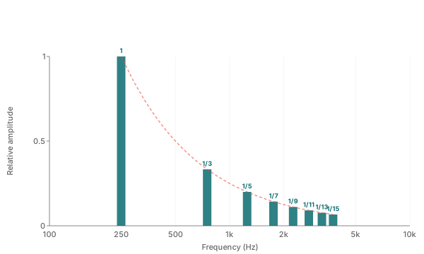
Figure 7.4. Fourier transform of the square wave shown in Figure 7.5.
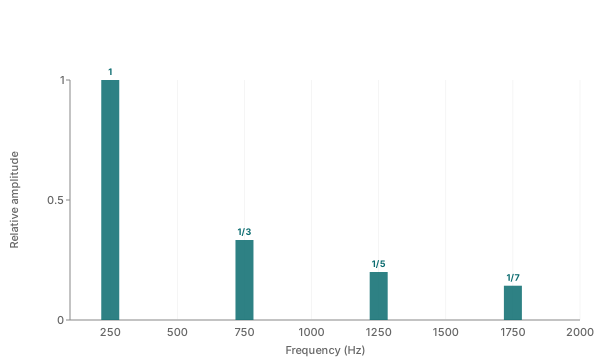
Figure 7.5. A plot of the relative amplitude of each harmonic component of a square wave, up to the seventh harmonic.
The fact that an FFT essentially “freezes time” makes it less useful for analyzing the temporal evolution of a sound source, although it is usually perfectly adequate for describing a filter or loudspeaker frequency response. In order to get an idea of the temporal evolution of the harmonic structure of a sound, multiple FFTs of a waveform can be taken over successive portions of time. These can then be displayed as in Figure 7.6; the relative intensity corresponds to the color intensity. Figure 7.6 shows both the time and spectral display of a piano note (left) and a cymbal (right). Click or tap each sound to associate the picture with the sound. Note that, in the piano sound on the left, the higher frequency spectral components die out relatively quickly compared to the lower frequencies; while in the cymbal example on the right, the higher frequencies of the complex spectrum are present throughout the sound’s decay.
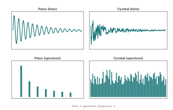
Figure 7.6. Time (top) and spectra (below) displays of a piano note (left) and a cymbal crash (right). Click or tap the buttons above to hear each example. Time is indicated on the x axis; the y axis is amplitude as a function of the quantized sample value (top) or level as a function of frequency from 0.1–9.0 kHz (bottom).
Still another way to view the time-varying nature of the spectral energy of a sound file is to take multiple FFTs and then arrange them in perspective — a waterfall display, as shown in Figure 7.7. This is also termed a perspective (time-level-frequency) graph.

Figure 7.7. Waterfall spectral display of the piano note. Each time slice (measured in point samples, or pts) indicates a separate FFT, which collectively show the evolution of spectra over the duration of the sound.
Figure 7.8: Live Spectrogram Waterfall
Real-time time-frequency-level waterfall. Each painted polyline is one FFT frame; newer frames sit in front, older frames recede in perspective. Pick a source — pre-rendered sample, song, a local audio file, a live microphone, or a MIDI file — and watch its spectrum evolve. The currently-active source is highlighted below.
Tip: the Play button toggles to Pause while playing (audio freezes, waterfall holds its current state for inspection); the separate Stop button halts and clears. The default piano source matches Fig 7.7 above — compare the static reference to its live equivalent. The microphone source shows the partials of a sung or spoken voice changing with each vowel; clap once to see a broad transient flash. The MIDI upload path uses an in-browser synth (no SoundFont), so the display shows the synth's spectrum, not the instrument the MIDI was authored for — useful for seeing exactly what a built-in additive triangle-wave voice produces.
Sound Modification Functions
It’s impossible to show every manner in which sound can be modified; else there would be no room for creativity. Sometimes simple but over-used techniques like playing a sound backwards (for example, a cymbal crash — , ; or a tuba — , ) can result in a seemingly stunning effect, but both trained listeners and the everyday public eventually recognize (and eventually get bored) by them. Nevertheless, simple is not necessarily bad. On the other hand, a multitude of complex parameters is available in a program such as Tom Erbe’s SoundHack , yielding either the most unique sound imaginable or something that sounds no better than backwards. The point is that sound modification is an art, requiring constant experimentation and sonic feedback. Below, we’ll sample both some common and unique ways for modifying sound.
Time Delay
One of the simplest yet most effective methods for altering a sound is to mix it with a time-delayed version of itself. This is usually done in tandem with changing the amplitude of the time delayed version. Figure 7.9 shows a two-channel sound file where the lower track is a time delayed, 50 % amplitude version of the upper track. If the delay is short — below around 20–40 ms, depending on the sound source — the difference between an unaltered sound file and one mixed with a time delayed version of itself will be heard as a change in timbre. Mixing so that the time delay is in a separate output channel from the sound source can change the spatial location and extent of the sound source as well. These effects result from the constructive and destructive phase interferences discussed in Chapter 3.
Delay effects are easily simulated with analog delay effects devices; with software editing programs, pasting a section of a silent sound file before a sound file track can be used to create the delay. In Figure 7.9, a monaural delay would be formed by mixing the two tracks, while a stereo delay is formed by playing the upper track out the left channel and the lower track out the right. In Figure 7.11, a table of sound examples is given. In particular, compare the sonic difference between the stereo and monaural delays over headphones.
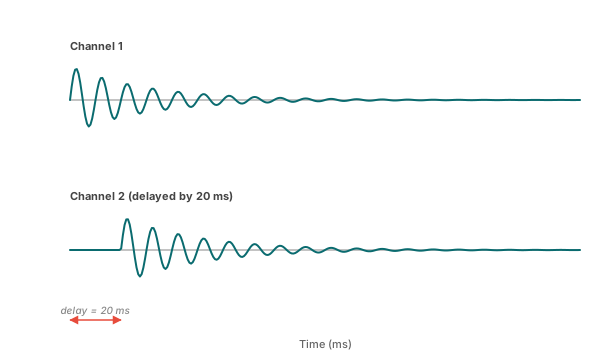
Figure 7.9. Time Delay between two sound file channels.
Figure 7.10: Delay & Echo
A single delay line with feedback. Short delays (< 20 ms) create comb-filter coloration; medium delays (40–200 ms) sound like slapback; long delays (> 300 ms) are echoes. Crank the feedback to hear taps repeat, and toggle ping-pong stereo to bounce them left/right. The echogram below shows each tap as a discrete spike — direct sound, then the first delay, then the feedback repeats — updating live as the parameters change.
Figure 7.11. Audio examples of adding time delay. Each grid’s rows step through three delay times; columns contrast mono mix (delay folded back into the source) with stereo (delay routed to the opposite channel). Compare a row across the two grids to hear how the same delay reads on tonal vs. broadband material, or a column down to feel how short delays act as comb-filter coloration, medium delays as slapback, and long ones as discrete echoes.
Filtering
Tone controls and graphic equalizers are types of audio filters. These modify the spectral balance of an input sound by selectively emphasizing some frequency components and de-emphasizing others. In Figure 3.2 the graphic equalizer was shown related to overall timbre; filtering was demonstrated in terms of its effect on a piano sound source.
Filters are used to remove or emphasize a region of spectral energy in a sound source. They can be used to alter the perceived timbre of a sound, or to remove unwanted aspects of a sound. For instance, many microphones have high-pass filters (HPF) that eliminate any frequency below, e.g., 75 Hz. This filter allows frequencies above 75 Hz (the pass band) through, while attenuating frequencies below this setting (the stop band). Rumble from HVAC systems, passing trucks, and other low-frequency vibrations that can seriously interfere with obtaining a clean recording and preventing distortion are attenuated; few sound sources have energy below this frequency. The high-pass filter B shown in Figure 7.12 has a cut-off frequency of 3 kHz; the pass band is above this frequency and the stop-band is below it. Filters A and C have cut-off frequencies of 1 kHz and 8 kHz, respectively.
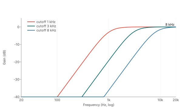
Figure 7.12. High-pass filter with cut-off at 1 kHz (A), 3 kHz (B) and 8 kHz (C).
Below the two filter explanations, a single 2×3 matrix compares the same cut-off frequency across high-pass and low-pass versions on the same noise source. (A low-pass filter (LPF) attenuates frequencies above its cut-off frequency; three low-pass filters — 1, 3, and 8 kHz — are shown in Figure 7.13.)
Reference:
Listen down a column to hear what the same cut-off does to noise from opposite ends of the spectrum; listen across a row to walk the cut-off from narrow to wide for either filter type.
Often, there is not sufficient energy above a certain frequency from the sound source; the overall noise level can be reduced by filtering above this point. Listen to the unaltered bongo sound and then with a low-pass filter — notice that the sound is still recognizable, but sounds much cleaner. At the same time, some high frequency information has been lost.

Figure 7.13. Low-pass filter with cut-off at 1 kHz (A), 3 kHz (B) and 8 kHz (C).
Another type of filter acts only on the spectrum within a certain region: a band-pass (BPF) filter passes a chosen band and attenuates what lies outside it, while a band-stop (BSF) filter attenuates the chosen band and passes the rest. Figure 7.14 shows two band-pass filters, with center frequencies of 3 kHz and 9 kHz; and a band-stop filter with a center frequency of 12.5 kHz. The center frequency is the midpoint of the frequency band that is not attenuated (for a band-pass filter) or the midpoint of the frequency band that is attenuated (for a band-stop filter). The bandwidth refers to the width of the spectral region that is passed or rejected, usually measured between the -3 dB (half-power) points.
These filters are the basis of graphic equalizers (EQs). We have indicated the cut-off frequency as the midpoint between the pass band and stop band. No filter can have a perfect transition between stop band and pass band; there is always a transition band — the range of frequencies over which the response moves from one to the other. How steeply it moves is the filter’s slope, quoted in dB per octave or dB per decade. But the quality of a particular EQ is partly a function of how narrow the slope is, and the minimum size of the bandwidth. Equalizers that came with the software editing tools of the period had wide bandwidths and broad slopes, allowing real-time modification of a sound for auditioning at some cost in precision compared with an outboard analog or digital equalizer. That trade-off has since disappeared: a software equalizer is limited by the filter it implements and the cycles available to run it, not by being software, and arbitrarily steep and narrow filters are now ordinary. The band-pass filters in Figure 7.14 would be considered less accurate than the band-stop filter, due to the differences in the narrowness of the slope.
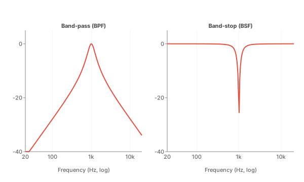
Figure 7.14. Band-pass (red, blue) and band-stop (light blue) filters.
Filter Playground
Apply a biquad filter to any source and see its frequency response (the white curve) overlaid on the live spectrum (the teal area). Drag the cutoff and Q sliders to reshape the spectrum in real-time. Try a low-pass on white noise to hear the brightness disappear; a band-pass on the piano picks out one resonance; a notch removes a single frequency.
Reverberation
Natural reverberation is the effect of an environmental context on the sound quality of a sound source. We are more aware of reverberation inside of the enclosed spaces that we occupy in daily life, but reverberation is also present in many outdoor situations. Only in anechoic chambers or in atypical environmental conditions, such as within a large, open expanse of snow-covered ground or on a mountain summit, are sound sources ever non-reverberant.
A sound source’s direct sound is defined as the wave front that reaches the ears first by a linear path, without having bounced off a surrounding surface. Reverberation on the other hand refers to the energy of a sound source that reaches the listener indirectly, by reflecting from surfaces within the surrounding space occupied by the sound source and the listener. Reverberation can be thought of as a large collection of time delayed versions of a sound source that decay in intensity over time as they arrive at the listener (see Figure 7.16).
The direct and time-delayed sounds arrive so quickly in succession after the initial waveform that they are perceived as one separate sound source, arriving from a single location defined by the direct sound (). However, if the reflection arrives late enough in time, it is heard separately as an echo (), similar to the simple time delay described above.
Reflected energy is categorized in terms of early and late reflections due to both physical and psychoacoustic criteria. The early reflections of a direct sound are followed by a more spatially diffuse reverberation termed late or dense reverberation. The process that carries one into the other is diffusion: each reflection scatters into several weaker ones, so arrivals multiply until they can no longer be told apart, and the room stops being a list of echoes and becomes a decay described statistically. These later delays result from many subsequent reflections from surface to surface of the environmental context. In a typical room, the buildup of successive orders of reflections begins to resemble an exponentially decaying noise function during the late reverberation period, causing individual reflections to be lost in the overall energy field.
Figure 7.17 shows an impulse response of a real room, obtained by recording a loud impulsive noise with an omni-directional measurement microphone. Figure 7.17 also shows identification of two possibly significant early reflections. Significant early reflections, those with a significant amplitude above the noise floor, reach the receiver within a period around 1–80 ms, depending on the proximity of reflecting surfaces to the measurement point.

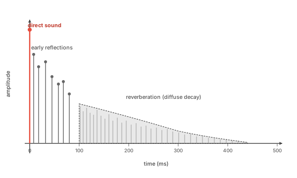
Figure 7.16. Top: Direct sound (blue) and early reflections (red). Below: reflectogram showing direct sound (green), early reflections (red) and reverberation (blue).

Figure 7.17. An impulse response measured in a classroom with an omnidirectional microphone. Time runs left to right and the vertical axis is amplitude; each vertical stem is one arrival of sound at the microphone. The first and tallest is the direct sound, having travelled straight from source to microphone. The stems labelled early reflections are individually countable arrivals, each one a distinct path off a wall, floor or ceiling. The reverberation tail is made of exactly the same kind of arrival — there is no second sort of event — but by then so many paths are returning, so close together, that they stop being separable by ear or eye and merge into a smooth statistical decay. The boundary is one of density, not of kind.
Figure 7.18: Reflection Explorer
Drag the source (+) and the sink (−, the listener) anywhere in the room, choose how many wall bounces to include, and the reflection paths redraw. Each path is the straight line from a virtual image of the source — the source mirrored in a wall, and then in another, and so on — folded back into the room at every wall it crosses. Click or tap Play to release one impulse per path: all leave the source together, travel at the same speed, and arrive at the sink at times set by their path lengths, populating the echogram below in arrival order. The 3D view shows the whole shoebox at once, mirrored in all six surfaces rather than four, so ceiling and floor bounces join the picture — order 2 rises from 13 paths to 25, and order 3 from 25 to 63. Dragging moves an endpoint across the floor; the two height sliders move it up and down. The room is treated as bare and rectangular, with omnidirectional source and sink and no diffraction or scattering, so the picture is cleaner than a real room. Each ray dims as it travels, standing in for the absorption and spreading that make a longer path arrive fainter. Swap source & sink exchanges the two. Helmholtz reciprocity says that running the path the other way — sink to source instead of source to sink — leaves the transfer function between the two points unchanged. Not only the path lengths are reciprocal but everything that multiplies along them: spreading, absorption at each surface, transmission, every reflection coefficient. Arrival times and amplitudes are therefore identical either way, so the rays are redrawn reversed while the echogram stays exactly put. Two ears replaces the single sink with a head: the ears sit 18 cm apart, facing wherever the sink orientation control points them, and each gets its own echogram — left drawn upward from the center line, right downward. Every reflection then arrives twice, at slightly different times and levels. The offset between a pair of spikes is the interaural time difference, the difference in their lengths the interaural level difference; both are read out for the direct sound. The rays are drawn to each ear in turn: solid and warm to the left ear, dashed and cool to the right. The ears are only 18 cm apart in a room metres across, so the two fans very nearly coincide — the dashing keeps them legible where they overlap, and either can be hidden with the Rays selector when the room gets busy. Each path launches two impulses, one bound for each ear; they leave together and arrive apart, which is the interaural time difference happening rather than merely plotted. The head carries a nose showing which way it faces, and head size sets the distance between the ears — 18 cm is about human, and widening it toward an elephant exaggerates both interaural differences until they are impossible to miss. (The separation is held to whatever fits the room, so an ear never ends up through a wall.)
Live echogram — amplitude against time at the sink. The dashed rule at t = 0 is the impulse leaving the source, not an arrival; the interval from there to the direct sound landing is the propagation delay (the time of flight, distance / c), and the gap from the direct sound to the first reflection is the pre-delay — the cue that tells the ear how large the room is before any tail has built up. At α = 1 the surfaces absorb everything, so nothing comes back and only the direct sound survives — an anechoic room, or equivalently no walls at all; at α = 0 they are perfect mirrors and every reflection returns undiminished by the surface. Each spike falls as 1/distance, by (1 − α) once per bounce off a surface, and by the air absorption over the meters it travels. The rays in the room above are drawn at the amplitude they still carry at each point, so raising either absorption dims and thins the beams as it shortens the spikes. Absorption is applied where it happens — at the surface, not gradually along the flight towards it — so a ray crosses the room at full strength and loses energy in a step each time it strikes something. With the surfaces fully absorbing, the beams therefore reach the walls undiminished and stop dead there: still energetic all the way to the boundary, and returning nothing from it. The echogram says the same thing on the time axis. A solid stem is an arrival — sound reaching the sink — while the small open marks before it are the moments that path struck a surface, drawn at the strength it carried when it got there. Raise the absorption and the stems shorten while the marks do not, because what the room takes away is the return, not the journey; at α = 1 only the marks and the direct sound remain. Every arrival plotted here is an early reflection — discrete and countable — which is why this axis spans tens of milliseconds where the measured response in Figure 7.17 runs to a full second. The dense reverberation tail of a real room is the sum of many thousands of paths at reflection orders far beyond the four offered here, so it lies past the end of this axis rather than being omitted from it.
The longer that it takes reverberation to decay, the larger the enclosure is perceived to be. This is related to the reverberation time control in software and hardware reverberators. This is probably the most perceptually salient aspect of natural reverberation. Changing the ratio of direct to reverberant sound (the R/D ratio) at the recording device is also a powerful cue, and can create powerful cues for auditory distance. This is because as we move away from a sound source, the level of the sound coming from reverberation remains more or less constant while the level of the direct sound is diminished.
What sets that decay time is how much energy each encounter with a surface removes. The absorption coefficient α is the fraction absorbed rather than returned: near 0 for tile or glass, which give almost everything back, and approaching 1 for thick carpet, heavy drape, or upholstered seating, which convert it to a little heat. It varies with frequency, which is why a furnished room sounds not merely quieter but duller — soft materials absorb treble far more readily than bass, and the tail that survives is the low end of it. The reflection explorer above uses exactly this quantity: its Surface absorption control is α.
Summed over every surface, absorption gives the room constant, R = S̄α / (1 − ᾱ), where S is the total surface area and ᾱ the area-weighted average absorption. It is what decides the level of the reverberant field, which settles at Ir = 4P / R and, unlike the direct sound, does not fall off with distance — the reason the R/D ratio works as a distance cue at all. Doubling the absorption halves the reverberant level, a 3 dB reduction, which is a sobering figure for anyone hoping to quieten a hard room by hanging a few curtains.
The R/D ratio is typically controlled on a hardware device (or its software-plugin equivalent) by the level of the effect control (the “wet” portion of the output of the device), relative to the level of the “dry” signal (unaltered portion of the signal). On an analog mixer, the level of the effects send and return controls is the way the R/D ratio is altered (see Figure 5.14 for an illustration of effect send and return). Sound examples were provided in Figure 5.13 on how changing the microphone distance and pickup pattern could alter the amount of reverberation. One way to simulate the R/D ratio using sound editing software is to crossfade across two versions of an audio file, one completely dry (anechoic) and one as wet (reverberant) as could possibly be wanted. By mixing the combination and altering the relative levels, reverb of the resulting sound can be smoothly controlled.
Often, the goal of reverberation is to provide just a small suggestion of room quality (“ambiance”) to a “dry” sound. A particular recording environment is often chosen for its reverberation characteristics (for the same reason people like to play music in stairwells and in subways). However, there is no reason to imitate natural reverberation; a myriad of effects can be created. One interesting effect involves placing sounds in unexpected reverberation situations, such as the little boy somewhere in an empty Taj Mahal ().
In the examples in Figure 7.19, a sound processed with different wet-dry (R/D) ratios can be compared and with different reverberation times. The reverberation was synthesized using a commercially-available outboard DSP device. The reverberation possible with basic software editing tools can be particularly disappointing. For instance, here is a sound reverberated with a “large hall” setting (), compared to the same sound reverberated using a studio-quality outboard reverberator (). On the other hand, the cutting-edge approach of combining 3D sound and reverberation techniques for auralization allows for the most realistic and potentially exciting results (see Chapter 9).
Figure 7.19. Reverberation time (columns: 0.3, 1.0, 2.5 s) and R/D ratio (rows: small vs. large reverberant-to-direct ratio) applied to the same Piano (left) and Speech (right) sources. Compare a row across the two grids to hear how the same reverb reads on tonal vs. broadband material; compare a column to hear the reverb length grow at a fixed R/D ratio. The unaltered source is at the top of each grid.
Three quite different methods go by the name. Algorithmic reverb builds a tail out of delay lines and all-pass filters tuned until the result sounds like a room; it is cheap, endlessly adjustable, and answerable to no particular building. Convolution reverb instead multiplies the signal by a measured impulse response — a recording of how one real space answers a single sharp sound — so it reproduces that space and no other, at the cost of being hard to alter afterwards. Physically modelled reverb computes the reflections from a geometric description of a room, which is what the auralization work in Chapter 9 does, and what lets a space be heard before it is built. The playground below is convolution, with one difference worth knowing: rather than a measured response it generates the impulse from the controls, which is why room size and decay can be dragged continuously when a real measurement would fix them.
Figure 7.20: Reverb Playground
Convolution reverb with procedurally-generated impulse responses (no IR files to download). Tweak room size (length of the impulse) and decay (how fast it fades) to morph between a closet, a vocal plate, a concert hall, and a cathedral. Pre-delay adds the initial “throw” before reflections arrive. The echogram below visualizes the impulse response as the parameters change — the tall spike on the left is the direct sound; the shaded gap is the pre-delay; the decaying tail is the convolved reverb. For the operation itself — how an impulse response and a signal combine, one shift at a time — see the Convolution Explorer, whose Click or tap ⊛ Room pairing is this demo in miniature.
Compression-Expansion
Audio compression-expansion is sometimes referred to as companding. As mentioned previously, the goal of audio compression refers to limiting the level of a waveform to a certain range that is narrower upon output compared to input. Expansion has the opposite goal; the purpose is to boost the level of an input signal that falls below a certain threshold. When used together, it is possible to narrow the dynamic range of a sound to a more limited range than it has normally. This is very important in broadcasting; one of the reasons a radio announcer’s voice sounds so consistent in volume is due to the use of companders. Almost all popular recordings are compressed as well, so as to sound good on a wide variety of equipment. Recall that the dynamic range of the playback environment is much narrower than that of the real world (see Figure 2.4). This also applies to down-quantizing a sound file from 16 to 8 bits, as discussed previously in this chapter.
Compression-expansion can be taken beyond a merely practical result. Figure 7.21 shows examples of an unprocessed and a compressed and expanded cymbal crash. Note that the quieter parts are louder, and the louder parts are quieter. Note also that the natural decay of the cymbal into the noise floor has been eliminated.
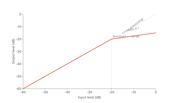
Figure 7.21. Effect of companding on the intensity of the signal. Click or tap on each example to listen to the effect.
The interface to a compander is complex. The best way to become familiar with the various parameters is to work with a real-time outboard device, or to spend time with a software plugin, until a sense of what is gained versus what is sacrificed develops. Figure 7.22 below shows a dynamics processing interface as both a skeuomorphic control surface (top) and explicit sliders (bottom) — the two are linked in both directions, so dragging the fader or rotating a knob updates the slider, and vice-versa. The “threshold” fader is probably the most important control. Compression occurs only when the signal goes above the level indicated (or, for expansion, when a signal goes below this level). The “detect” fader allows a transition between evaluating individual samples versus evaluating the mean value of a group of successive samples. “Attack” and “release” affect how quickly the effect is activated; its function is to smooth the effect of compression or expansion for a more natural sound. The “ratio” controls the overall amount of the effect. For compression, a 10:1 ratio means that a 10 dB increase in the input results in a 1 dB increase in output; for expansion, a 1 dB increase at the input results in a 10 dB increase in output.
Figure 7.22: Live Compressor
Audible dynamics processing with a skeuomorphic control surface. Drag the threshold fader up/down, or drag any knob vertically to rotate it. The sliders below mirror the same parameters and stay in sync. Hover any slider label for a tooltip explanation. Toggle Bypass to A/B compare unprocessed vs compressed.
Phase Vocoding: Pitch Shift & Varispeed
Some of the examples played in Chapter 4 showed that it is possible to greatly alter the character of a sound using a simple pitch shift. This technique is accomplished by playing back a sound at a lower or higher sampling rate than the original sound was recorded at. This is equivalent to changing the speed on an analog tape. Note that as the pitch is changed, the duration of the sound changes proportionally. For example the following sound () has an animal-like character, somewhat like a seal or a sea lion. It was produced by shifting the pitch of a lovebird call downwards by 2 octaves — 25 % of the original frequency ().
More creative pitch shift effects can be obtained by varying the amount of pitch shift over time. In Figure 7.23, the interactive demo applies a pitch shift that follows a chosen curve — sine, triangle, sawtooth, or ramp. The first three repeat at the chosen rate; the ramp is the odd one out, gliding once from the bottom of its range to the top and then holding, over a span the rate control sets — 0.5 Hz gives a two-second glide. The contemporary equivalent of the SoundHack pitch-shift function shown below: choose a built-in waveform and adjust its center, depth, and rate live.
Figure 7.23: Time-Varying Pitch Shift
Pick a source, choose a curve (constant / sine LFO / triangle / sawtooth / ramp), then set the center pitch (the curve’s offset, in semitones), the depth (how far above/below center the curve swings), and the rate (how fast the curve cycles, in Hz). The graph below previews the current curve continuously; the red line marks “now.” Slow + deep = obvious siren / seasick warbling; fast + shallow = vibrato. Constant ignores depth/rate and just shifts the whole sound by “center pitch.” This is varispeed (tape-speed) pitch-shifting — duration changes with pitch.
We pointed out that pitch shifting alters the duration of a sound file proportionally. But what if the pitch of a sound is to be shifted without changing its duration? Or, conversely, change the duration but not the pitch? A process known as phase vocoding is a way to accomplish this.
Phase vocoding (termed pitch shift or time compression-expansion in some software packages) involves a non-real-time, computationally-intensive analysis-synthesis technique. The analysis involves calculating the waveform’s spectral energy via a series of band-pass filters, in a time-to-frequency analysis. This can be thought of as a series of FFTs that occur over the duration of the sound file. Once the signal is analyzed, it is possible to synthesize the original input signal via a frequency-to-time operation known as an inverse FFT. The advantage of the process is that during synthesis, parameters can be altered to result in time change without pitch shift, or pitch shift without time shift.
Best of all for producing special effects, the phase vocoder requires an exact, usually unpredictable set of parameter adjustments to create a “perfect” unprocessed-sounding result. Usually, some artifacts remain from the analysis-synthesis procedure; these artifacts can be in fact exploited for their own contribution to the effects, for instance, by setting parameters to below recommended limits. These parameters include the amount of overlap and the number of filters that occur during the analysis stage. Some software simplifies these parameters into a simple “quality versus processing time” slider control.