Storage: Miking and Recording
How to capture sound sources using microphones, understand directivity patterns, manage miking distance and reverberation, and route signals through a mixer.
Recording and Storage
Once sound sources have been chosen to function as cast members within a composition, it’s possible to move on to the task of recording (capturing) the sounds.
Figure 5.1 summarizes the chain of events in the recording and playback of desktop computer audio. An analog waveform (shown in red) is transduced into an electrical signal by a microphone. A pre-amplifier within a mixer or within the audio interface itself is used to amplify the signal from “mic level” to “line level.” The A-D converter causes the analog electrical waveform to be sampled at discrete intervals into a series of numbers that represent the sound, and then stores these numbers onto the hard disk. Once in the digital domain, the samples can be passed through a DSP (digital signal processing) stage — filtering, mixing, equalisation, effects, dynamics — before reaching playback. For playback, the numbers are converted back to an analog electrical signal by the D-A converter. The power level of the electrical signal is then boosted by the amplifier. The loudspeaker transduces the electrical signal into an acoustic, analog waveform, which differs from the input according to the distortion and processing of the recording-playback chain.

Figure 5.1. Chain of events in recording and playback of digital audio in a DAW.
Microphone Construction
For most purposes, a pressure transducer, or microphone, is the most important device for recording sound sources. Two of the most common types are the dynamic and condenser microphones. Dynamic microphones function via the movement of a wire known as a voice coil that is attached to the microphone diaphragm; these are mounted near a magnet (see Figure 5.2, left). Sound waves impinge upon the diaphragm, which is flexible. This moves the voice coil back and forth with the magnetic field, causing an electrical variation proportional to the incoming sound wave.
A condenser (or electrostatic) microphone works with an electrically-charged diaphragm located near a fixed, electrically-charged surface called the back plate (see Figure 5.2, right). The diaphragm and back plate together form complimentary parts of an electrical capacitor. Unlike a dynamic microphone, a voltage supply must be supplied to the condenser microphone. On less expensive microphones, such as those built into portable video cameras or smartphones, the voltage is supplied by a small battery inside the body of the microphone itself. An external power supply is necessary with professional microphones, which is provided from the mixing console or a specialized microphone preamplifier. This microphone voltage is sometimes referred to as phantom power since it can be delivered via the microphone cable; voltages usually range from 12 to 48 volts.
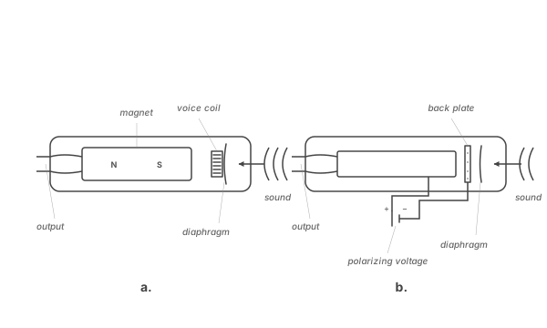
Figure 5.2. Cut-away view of dynamic (a.) and condenser (b.) microphones.
The choice between a condenser and a dynamic microphone depends upon several factors. Generally, condenser microphones have a wider, more linear frequency response than dynamic microphones, especially at high and low frequencies. Another issue is that dynamic microphones are generally more rugged than condenser microphones. This causes them to be the choice in sound reinforcement applications; a dynamic microphone can be dropped on the floor and still function nicely, whereas a condenser microphone tends to be more delicate. Condenser microphones also tend to have more features, such as a variable pick-up pattern, and filtering. Finally, condenser microphones are more liable to distortion than are dynamic microphones. For example, since percussion puts out very high dB SPL levels when played, one almost always uses dynamic microphones on them.
to listen to an example of speech recorded with a dynamic microphone, and to listen to an example recorded with a condenser microphone. Note that the condenser microphone has a fuller sound quality. The condenser microphone in this example is a professional-grade model (Figure 5.3, right), while the dynamic microphone is a widely used workhorse model (Figure 5.3, left).
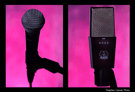
Figure 5.3. Dynamic (Shure SM-57) and condenser (AKG 414-EB) microphones.
A cymbal recording usually wants as much high frequency as possible, while a voice recording may not; the filtering of high frequencies is sometimes heard as a “warm” sound. In a recording studio, each microphone can be tailored to a particular recording technique to shape the tone color and avoid distortion. The differences between manufacturers, models, and even the internal electronic circuitry cause each microphone — even of the same kind — to sound at least slightly different from every other.
Below, we go over the most common types of microphones, with particular attention given to their directivity pattern (or “pick-up pattern”). It is common practice to describe a microphone primarily in terms of its directivity, and to identify it as a condenser or dynamic microphone.
Microphone Directivity Patterns
Two of the most common types of microphone directivity patterns in use are omni-directional and cardioid. An omni-directional microphone picks up a sound source equally from all directions, while a cardioid (sometimes called “unidirectional”) microphone is most sensitive from the front, and is progressively less sensitive towards the direction of the rear of the microphone diaphragm. Both — along with the narrower super- and hyper-cardioid patterns — are visible in the Polar Pattern Sandbox below. Their full three-dimensional generalization — the same directivity patterns expressed as spherical harmonics, as used in first- and higher-order Ambisonics — is explored in the Spherical Harmonics Explorer.
Figure 5.4: Polar Pattern Sandbox
Microphone directivity (指向性) follows the standard limaçon family:
gain(θ) = |(1−α) + α·cos θ|n, where n is the order of the pattern.
Drag the sliders or click or tap a preset to morph through omni, cardioid, supercardioid, hypercardioid, and bi-directional patterns. The mic capsule sits at the center and points up (0° = on-axis); concentric rings mark 25 % / 50 % / 75 % / 100 % sensitivity.
The directivity index (DI) reported below the plot is the ratio (in dB) of on-axis sensitivity to the spherical-average sensitivity: 0 dB for omni (no directionality), ≈ 4.77 dB for cardioid, ≈ 5.71 dB for super-cardioid, ≈ 6.02 dB for hyper-cardioid. Higher DI = more focused beam.
Pattern: Cardioid · DI: 4.77 dB
gain(θ) = |0.500 + 0.500·cos θ|
| Preset | α (cos-coeff.) : 1−α (const.) | DI (n = 1) | Special property |
|---|---|---|---|
| 0 : 1 | 0.00 dB | No directionality (spherical pickup) | |
| ⅛ : ⅞ | 1.13 dB | Broader than cardioid (gentle rear rolloff) | |
| ½ : ½ | 4.77 dB | Exact null at θ = 180° | |
| ⅝ : ⅜ | 5.67 dB | Approx. max front-to-back ratio; nulls at ±126.9° | |
| ¾ : ¼ | 6.02 dB | Max DI over first-order family; nulls at ±109.5° | |
| ⅞ : ⅛ | 5.67 dB | Past DI maximum — mirror of Super in α | |
| 1 : 0 | 4.77 dB | Nulls at ±90° (bidirectional) |
Note on order: the DI column shows values for first-order patterns (n = 1), which is what a single directional capsule can achieve. The theoretical ceiling at n = 1 is 6.02 dB (hyper-cardioid). Higher orders — n = 2, 3, 4 — are what raising that first-order pattern to a power gives: an abstract directivity model rather than a description of any particular microphone. They raise the ceiling to n = 2: 9.54 dB, n = 3: 12.04 dB, n = 4: 13.98 dB. The live DI readout below the polar plot reflects the currently selected n.
Tip: raising the order n above 1 narrows the main lobe, giving the polar shape a higher-order system would produce. It is a mathematical narrowing, not a recipe for building one: a shotgun microphone does not work this way — see the interference-tube discussion below — and the same polar curve can be reached by quite different physical means. The absolute-value in the formula collapses what would be the negative rear lobe back into a positive magnitude — which is why α = 1 yields the symmetric figure-8 instead of a single front lobe. The colon notation (e.g. ½:½) reads α : (1−α) — the proportion of cosine vs. constant term.
Try this: (a) Sweep α slowly from 0 to 1 with order fixed at n = 1: watch the omnidirectional circle dimple at the back to become a cardioid, then pinch into the two-lobed figure-8. (b) Snap to Cardioid, then step n from 1 to 4: each integer step compounds the first-order pattern with itself, narrowing the main lobe. Cardioid DI follows 10·log₁₀(2n+1): 4.77 → 6.99 → 8.45 → 9.54 dB across n = 1…4 — per-step gains ~2.2, 1.5, 1.1 dB (diminishing returns). The narrowing is a property of the curve, not of any one construction: the same shape may come from a capsule array, from a horn, or from beamforming in software. (c) Compare the back-rejection at α = 5⁄8 (supercardioid) vs. 3⁄4 (hypercardioid): the hyper is more directional but has a bigger rear pickup lobe — the classic trade-off between front-focus and rear-rejection that drives microphone choice.
Figure 5.5 (left) shows a bi-directional (sometimes called “figure-8”) microphone pattern. Usually, the bi-directional pattern is a selectable feature of a microphone that has the capacity for switching between several different patterns. This type of microphone is equally sensitive from the front and rear, but attenuates signal from the sides, making it very useful for specialized situations such as miking a conversation between two people. It can also be used to emphasize reverberation in a more specific manner than an omni-directional microphone, as demonstrated in Figure 5.13, below.
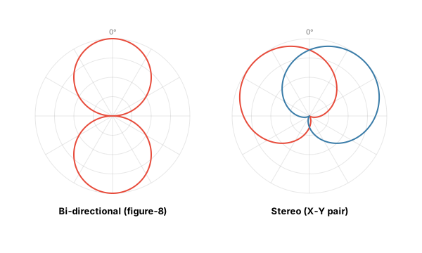
Figure 5.5. Bi-directional (left) and stereo (right) miking patterns.
Figure 5.5 (right) shows a type of stereo microphone pattern. A stereo microphone contains two microphones in a single housing with two separate output lines. One line is usually sent to the left input and the other to the right input. These tend to be either relatively inexpensive or very expensive condenser microphones. The less expensive models are designed to be used for ensemble as opposed to spot miking, and have two cardioid-pattern microphones, sometimes with a range switch that moves the pickup pattern outwards from 90° to 120° to allow capture of a wider range of sound sources. The more expensive, professional-level stereo microphones have variable patterns that can be adjusted electronically. Figure 5.6 shows a photograph of a medium-quality stereo condenser microphone.

Figure 5.6. Stereo cardioid microphone with variable cardioid pattern.
Figure 5.7: Stereo Mic Techniques
Four canonical pairings, simulated. A virtual source moves left/right (manual slider or auto pan); each technique converts source angle into L/R signals using its own model. Listen on headphones — the differences in stereo width and center solidity become obvious. The vectorscope (lower right) plots L vs R: a vertical line means in-phase mono, a horizontal wedge means out-of-phase.
Beyond the basic cardioid, two narrower patterns are common on professional microphones: super-cardioid and hyper-cardioid. The super-cardioid pattern is often a selectable feature on more expensive microphones, and allows a tighter focus on sound from the front compared to the sides — though the response increases a bit from the rear of the capsule. The hyper-cardioid pattern is narrower still, with a correspondingly larger rear pickup lobe. Both are visible (and freely morph-able) in the Polar Pattern Sandbox above; the DI column there reports each preset's directivity index.
A shotgun microphone is used to aim the pickup pattern as precisely as possible. Its directivity does not come from the polar mathematics above. A hyper-cardioid pattern is a first-order pattern and needs no particular body shape; short pressure-gradient capsules produce it routinely. What makes a shotgun a shotgun is the slotted interference tube ahead of the capsule: sound arriving on-axis travels straight down the tube, while sound arriving off-axis enters through many slots along its length, so those contributions reach the capsule by paths of differing length, arrive out of step, and partly cancel. Because that cancellation depends on the ratio of tube length to wavelength, the effect is strongly frequency-dependent — which is why real shotgun polar plots grow side lobes at high frequencies instead of forming a clean beam. However, contrary to its portrayal in certain films, the pickup pattern is not so precise that it can be aimed at one sound source to the exclusion of all others. Shotgun microphones are used for an effect similar to close miking but are required to maintain a distance from the sound source, such as in some film and video shots.
Other Types of Microphones; Connections and Cable
We’ve gone over the most common types of microphones, but there are many other types with different methods of transduction, pick-up patterns and sizes that are appropriate for various applications. One that is especially useful is the miniature microphone, a small microphone that can be attached directly to the clothing of a person or to a sound source (some types are called lapel microphones since they attach to the lapel of a coat). These small omni-directional microphones can sound excellent when placed near the sound source, but are generally too noisy to use for distant miking. Studying a good source book on recording engineering techniques (see Chapter 7) and a catalogue from a microphone manufacturer is the next best thing to actual “hands-on” and “ears-on” experience.
Another issue is microphone impedance. Impedance can be thought of as electrical resistance; with longer distances between the microphone and the recording device, less resistance is desirable. Professional microphones are generally low impedance, and use 3-pin XLR connectors and shielded cable to provide noise immunity; the cable can be detached from the microphone (see Figure 5.8). “Consumer” microphones use either 1/4 inch or miniature phone jack connectors, and the cable is permanently attached to the microphone (see Figure 5.9).

Figure 5.8. XLR connectors. These are typically used with low-impedance microphones and shielded cable.
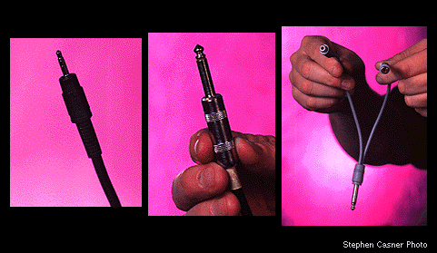
Figure 5.9. Connectors: stereo 1/8” miniature plug; 1/4” phone plug; “Y” cable — 2 RCA female connectors to a single 1/4” phone plug.
Microphone Distance and Reverberation
Three of the main considerations to miking distance are: 1) desired pickup pattern; 2) inclusion or exclusion of reverberation; and 3) avoiding distortion.
The ideal distance to a sound source depends strongly upon both the environmental and recording contexts. Spot miking refers to the technique of isolating a particular instrument, voice or other sound source with (usually) a single microphone placed relatively close to the source. Often several spot microphones are used at once, such as in sound reinforcement at a live concert, or in a recording studio. The recording and live sound engineers require the signal from each instrument to be as isolated as possible at the mixer, to enable independent adjustment of the level of each instrument. This is illustrated in Figure 5.10. An audio mixer is used to distribute each microphone input to left and right outputs that create the illustrated spatial imagery for the headphone listener.
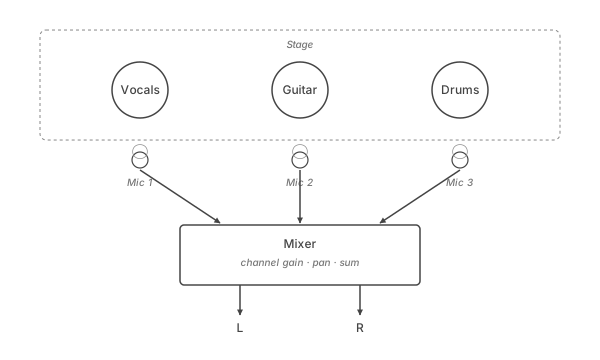
Figure 5.10. Close miking using cardioid-directivity microphones.
Distant miking refers to the technique of using one or more microphones to capture a group of sound sources and/or to capture the environmental context of a sound source. It is usually more difficult to accomplish good distant miking. Figures 5.11 and 5.12 show two different techniques. The first is referred to as “spaced omnis”; often a “hole in the center” of the speakers is perceived during stereo playback. The second is referred to as coincident pair miking. This technique is generally preferred, especially with classical music. A combination of microphones can also be used, but the chances of destructive phase interference as discussed in Chapter 3 become more relevant.
Note that in Figure 5.12 the image positions are reversed inside the head of the listener. This is because the left microphone is pointed at the right, and vice versa. The engineer could easily remedy this by switching the input cables to the mixer! But like photographs which are frequently reproduced with a “backwards negative,” stereo sound is often reproduced in reverse channel configuration, usually without negative effects. If a visual and auditory image were linked, this would naturally be a more noticeable problem.
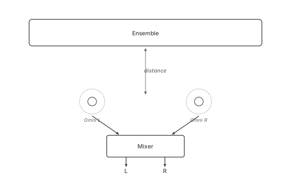
Figure 5.11. Distant miking technique using spaced omni-directional microphones.
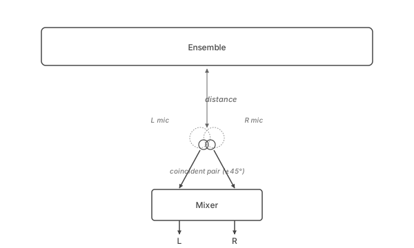
Figure 5.12. Distant miking technique using coincident pair (see text).
If there are undesirable sounds in the immediate vicinity, for instance the sound of a camera crew during a live shooting, then spot miking is always desirable. One of the first things that amateur recording artists as well as amateur photographers find out is that what they record usually has a lot more information in it than they desired, information that can detract from the intended image. A sound can be recorded at a cafe of some nearby people talking with a laptop’s built-in microphone, but the wind, other conversations, the dishes clanking, and so on will also be captured (for an example ). Our hearing system allows us to focus in on a desired signal more easily than a microphone, and since the recording system is both less precise and removed in time from our current associations, context, etc., the conversation becomes lost within the surrounding conversations.
That unwanted background has a second life, though. A location’s own quiet — ventilation, a compressor cycling, traffic through glass, and the room’s response to all of it — is called room tone, and it is worth capturing on purpose: thirty seconds to a minute at every setup, with the same microphone in the same position at the same gain as the dialogue, everyone present and still. The editor needs it. A cut between two takes is also a cut between two slightly different backgrounds, and the join announces itself; a continuous bed of room tone underneath hides those joins, fills the holes left where a cough or a passing airplane was removed, and supports dialogue re-recorded later in a studio, which arrives carrying no location sound at all. Cutting instead to digital silence does not read as quiet but as a fault, the background dropping away where the ear expects it to continue. And because every space differs in its noise floor and in the modes that color it, a bed borrowed from another location rarely passes — which is why room tone is gathered where it is needed, while the crew is still there.
The effect of reverberation within a room will indirectly affect the quality of a recording, even with close miking. We can alter the amount of reverberation either by moving the microphone or by changing its pick-up pattern. Figure 5.13 demonstrates this with a recording of a musical pattern played on the tablas. Position 1 is spot miking; an omni-directional microphone is used, with the mic placed almost in-between the tablas. Position 2 uses four different patterns at a distance of 3 feet; position 3 uses two different patterns at 6 feet. Listen closely to the differences (headphones are best), particularly to the differences in timbre and reverberation.
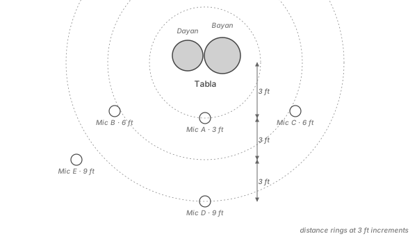
Figure 5.13. Tabla miking example (see text). Each black arrow corresponds to 3 feet distance. Click or tap the buttons below to compare miking distance and directivity differences.
While miking at different distances can result in different reverberant-direct sound ratios, bringing microphones up very close to a sound source can emphasize low frequencies in the spectra, sometimes in a very unnatural way. This emphasis is known as the proximity effect, and is frequently exploited when recording narratives in order to give the spoken voice a deeper quality ( to hear without proximity effect; to hear it).
Level Matching and Mixing
Besides microphones, electronic analog sound sources can serve —the output of a mixing console, another recorder, guitar pickup, or synthesizer— as sound cast members. In these cases there is a transference of electrical voltage from one storage medium to another. In most cases the device in question will have an output voltage level referred to as line level. Microphones on the other hand have very small levels and require pre-amplification so as to reach line level. Most audio interfaces work best when supplied with a line level input at the A-D converter, since the quality of a microphone preamplifier is a significant factor in the resulting quality of the input signal.
In order to pre-amplify and attenuate various microphone and line-level signals, a hardware, analog audio mixing console (popularly termed a “mixer“) is often the best choice. To the beginner, a mixer can look daunting with its many knobs, sliders and switches. A mixer is often described in terms of the number of inputs and outputs; e.g., an “8 in 2 out” configuration is quite common. It is easier to think of it as altering the audio signal flow from input to output much in the same way a plumbing system routes water in a house to various faucets. The key to understanding is in terms of the basic signal flow functions shared by all mixers. These are input gain controls, panning and output assignment, effect send and return, and output gain (or master gain) controls.
Figure 5.14 graphs each of these functions within a hypothetical, 2 input, 2 output mixer. The input gain controls scale or amplify the input signals in relation to one another. The signal is then passed to the output buss line; there is at least one buss line per output. If there are two outputs (a “stereo mixer”) then the pan control assigns the relative proportion of signal that is passed to each output buss line. The pan control is a simple way of controlling the stereo image at the output; panning to the center sends an equal level to both speakers, creating a “centered image;” images are shifted to the left and right proportional to the pan pot setting. The output of the mixer is a line level “mixture” of all of the input signals at each buss, which can then be connected to the input of an audio interface on a computer, a recorder, or a sound reinforcement system. The effects send and return is the way reverberation and other effects from external devices are added to each input.
An analog audio mixer such as described here can be a useful device for mixing signals as well as for providing pre-amplification for a microphone signal. But in many cases it is more convenient to use software mixing functions for DAWs and other audio software. These are described below in Chapter 7.
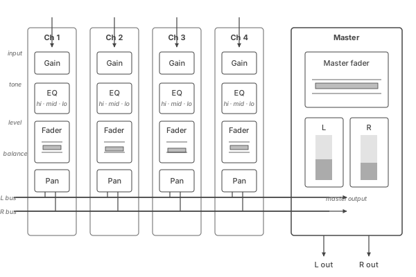
Figure 5.14. Functions of a basic mixer for digital audio in a DAW.