Audio Basics I: Communication, Frequency, and Pitch
How sound travels from source to listener, how we measure and perceive frequency, and why two nearly identical pitches create audible beats.
Introduction: Sound, Computers, and Media
This is an introduction without the usual spiel of what is media? or why is media production important? or let’s feel the excitement of the new age of computing. This site is about sound on computers, not about a specific version of a particular software product. Otherwise, had it been a “how to” site with a title like “All About Sound for XXX Software Package,” it would be worthless in a year or two. This is not so much a traditional site as it is a website with built-in audio examples. It is designed to be an integral part of learning for those who are either relatively new to the concept of digital audio or who want to know more than what they learned from the manual that came with their audio interface. The reader should finish this site with an increased appreciation of the fact that audio production is one of the most critical components of the multimedia phenomenon.
What makes working with sound for video, games, and interactive media so interesting is that it’s a relatively new, undeveloped medium, with a lot of room for originality. At the same time, production audio composition is extremely referential, to both the history and the contemporary scope of audio-visual communication, and electronic music in particular.
Hardly anyone would argue with the importance of audio in a media production, or with its power to influence the interpretation of a sequence of visual images. For instance, different compositional approaches to coordinating visual material to music, sound effects, and narration can give an entirely new context for interpretation.
Those last two italicized sentences were read without any audio accompaniment. Now re-read them after clicking or tapping . This is a kind of worker bee ostinato music useful in business presentations that gives a slightly aggressive quality to the text.
Now re-read the boxed paragraph after clicking or tapping . The feeling given to the text is by contrast much less serious, almost relaxed.
Now re-read the boxed paragraph after clicking or tapping . The feeling is even less serious (to say the least!).
A lot of the emotional feeling supplied by these different BGM (background music) accompaniments are culturally based due to television, film, and other mass media that effectively codify certain visual-audio relationships. But sound for media is not just about plugging in a certain code or method; there’s a world of subtle and artistic renderings that come from a real involvement in audio production. High-quality audio will actually make people report that games have better pictures, but really good pictures will not make audio sound better. Even if a media producer doesn’t take on the actual duties required for audio production, they can benefit from a thorough knowledge of the topic. The material in this website is designed to help make this possible through listening as well as reading.
Increasingly, the media producer desires to take on production chores previously reserved for specialists. In the traditional paradigm for producing an opera, one of the grandparents of audio-visual media, there is a specialist for the music (the composer), a specialist for the lighting, a specialist for the costumes, a specialist for the dialogue and story line (the librettist), and so on. Due to the scale of the resources that need to be assembled, an opera couldn’t exist without a multitude of players. Since a comparable media experience can now be produced on a laptop with a single program such as a modern DAW (Ableton Live, Logic Pro, Reaper), the centralization of duties is much more desirable and allows for more creative control over the end product. More than likely, the distinction between graphics and audio specialists in modern media will steadily diminish. Creators should aim to be as expert with the tools for sound as for any other media-production technique.
While opera, theater, and dance are obvious historical and contemporary manifestations of the integration of audio and visual media, the most influential of all media forms is probably commercial television production, both programs and commercials (assuming that it’s possible to make the distinction). The television industry is driven by commercial sponsorship and the same basic motivation that drives the computer, telecommunication, and entertainment industries: achieving popularity by capturing the imagination of the buying public to increase market share.
Since processing speed, memory, and graphics capabilities of computers continuously become less expensive and more accessible, a media form that was exciting two years ago must be superseded by something more profound, something perceived as an improvement to satisfy the inherent frustrations with what we have. Anything popular requires constant re-manufacturing and updating so as to rekindle the excitement. What better medium than the personal computer, which will only become increasingly pervasive in society?
Much is made of words like interactivity in describing interactive media, but people are discovering that certain types of interactivity slow the reader down, drive them to distraction, and send them looking for a good book. To summarize, it’s important to see beyond the hype and those features that seem attractive at the moment. Better than latching onto the latest bandwagon is to improve a knowledge of the basics, so that the content of the production can be as rich and unique as possible. Determining when and where sound is appropriate is more important to the art of sound design and composition than having an extensive library of sound effects. And that is what the rest of this website offers. Let the ears become as educated as the palate of a gourmet cook; it’s just as fun!
We’ll refer throughout this website to the person who takes on the role of audio production as a composer. The word sound designer could be used instead; the traditional distinction is that a composer makes music, while the sound designer does all other forms of audio, but the distinction is pretty useless since the definition of what constitutes music is in the ear of the beholder.
The Audio Communication Chain
A distinction must be made between everyday hearing and specifically listening to an audio reproduction system. Hearing sounds in everyday situations with our ears uncovered, our head moving, and in interaction with other sensory input can be called natural hearing. In daily life, thousands of vibrating sources contribute to a constantly changing soundscape that is available to our hearing system at every moment for analysis and interpretation. Amazingly, we’re able to hear out a desired sound from the cacophony of stimuli that is constantly presented to us, such as listening to a conversation in the midst of busy city traffic, or concentrating on the oboe in an orchestra while sitting in an audience with people coughing, whispering, and rustling about.
By contrast, listening to electrically produced sound could be termed virtual hearing since the acoustic imagery is not from an actual sound source, but instead is produced electrically by a sound system and stereo headphones or loudspeakers. Virtual hearing with a sound system involves a limited number of individual sound sources chosen deterministically to create a specific message within a medium.
Unlike everyday communication in the context of natural hearing, there is a more predictable situation within a media application. The visual attention of the user and what they’re doing at a moment in time can be pretty well estimated. The control over a virtual hearing sonic experience is characterized by the composition of sound, with a media product produced by an author specifically for that context. The author desires to communicate a specific experience to the user of a media work, with a degree of planning not unlike a traditional staged theatrical experience, where lighting, sounds, and characters are all carefully planned in their presentation to the audience. A further difference is that the virtual sound sources are produced exclusively by a sound system, with digital storage and playback devices being the norm for production audio.
It is very important to realize that virtual hearing is not necessarily equivalent to natural hearing any more than an image on the television screen represents reality. A composer formulates a particular reality that attempts to influence the user to ignore most of their natural hearing experiences at a given moment. The degree of immersion of a particular production audio experience can be defined in one way as the degree to which virtual experiences eclipse natural experiences, pushing them out of the consciousness of the user. On a computer, the challenge is to make the audio at least as immersive as it normally is when listening to a high-quality stereo system. In other words, if it’s good enough so that the user is transported, no matter how briefly, the user will want to experience the entire message communicated by the composer.
The creation of a virtual acoustic image that exactly matches a particular natural one is arguably impossible, but luckily for the recording, broadcasting, and telecommunications industries, it is less difficult to come up with a convincing match compared to the visual world. Nevertheless, the more a composer considers each of the components in detail in the communication chain shown below in Figure 1.1, the better the end product.

Figure 1.1. The communication chain for production audio.
The audio transmission path from author to listener shown in Figure 1.1 can be described according to a chain of events within the broader categories of a source, medium, and receiver. The source is one or more acoustical or electrical sound sources, such as a spoken voice for narrating a story; a musical passage that exists on another electronic format, such as an audio file or streaming source; or any particular sound that one wishes to capture.
The medium involves three steps: the storage of an acoustical or electrical signal into digital form; transformation of the digital signal; and, ultimately, conversion back from digital to analog form for playback of the signal. We need to convert between acoustical, electrical, and digital representations at several different stages within the medium. This conversion is accomplished by a transducer, a physical device used to change energy from one form into another. A pressure microphone is a transducer used to convert acoustical to electric energy at the source; a loudspeaker is a transducer for converting electric into acoustic energy.
The receiver is comprised of the listener’s hearing system, their immediate perceptual responses, and their higher-level cognitive processing. We can customize a composition for a single receiver, ourselves, or a particular loved one, but most people compose with an awareness of a target audience.
Each element of the communication chain breaks down into a number of physical, electrical, neurological, or perceptual transformations. This is represented in the abstract by the sections numbered 1 through n in Figure 1.2. Each transformation compounds with the others, and can be desired and/or undesired. It is absolutely certain that some sort of mismatch will occur as a result of the process. These can be due to a wire, a digital signal processor, or a room, and all will affect the communication of the identification, timbre, and spatial location of a sound source from the beginning to the end.

Figure 1.2. Each transformation contributes to a mismatch between intent and result.
Now we will detail each stage of the communication chain as it typically applies to the production of production audio. In subsequent chapters, some of these stages will be investigated in more detail, particularly those that occur within the digital domain of audio production for video, games, and interactive media.

Figure 1.3. Components of the communication chain in production audio: sound sources and transduction into the digital medium.
The source can begin as an acoustical or electrical signal, as shown in Figure 1.3. The goal is to capture these sounds using some form of transducer for eventual digital storage within the digital medium of a desktop computer. The most common and familiar method for transforming acoustic sources is to use a microphone that will respond to variations in air pressure. These are the most familiar types of microphone.
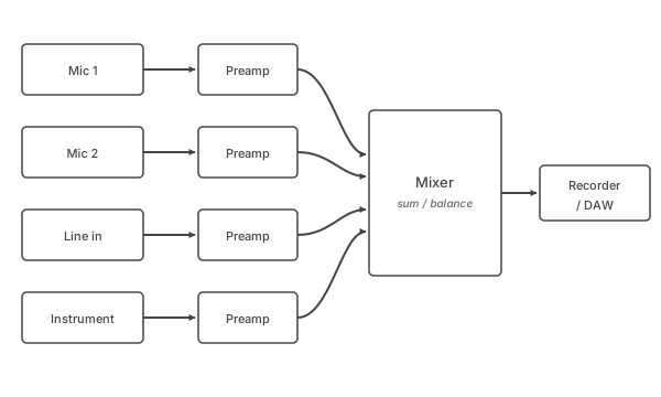
Figure 1.4. Pre-amplification and mixing.
Many sources, especially acoustic instruments, are effectively transduced with a contact microphone, typically attached to a sound board of an instrument, responding to vibration rather than pressure. Other possible transducers include the magnetic pick-ups of an electric guitar.
All of these transduction methods end in an analog electrical signal, but they do not all begin in the same place: a pressure microphone responds to acoustic pressure, a contact microphone to mechanical vibration, and a magnetic pickup to the motion of a steel string through a magnetic field. Other transformations can occur as well, as shown in Figure 1.4. We more than likely require some sort of re-amplification before reaching the computer, since there will be a mismatch between different levels, and the signal from an electric guitar pickup or microphone is quite minuscule. There might also be an analog audio mixer present to blend several sounds together before going to the computer. Additional signal processing in the form of effects or equalization may also be involved. However, some sources, such as a synthesizer or sampler, are already in analog or digital electrical form. In many cases, the source is a previously captured acoustic or electric signal that exists within a digital storage medium — or, increasingly, generated outright by an AI or generative-audio model (text-to-speech, neural-network voice cloning, generative music systems, denoising or restoration networks). Figure 1.5 shows the most common families of source available today.

Figure 1.5. Common source families for production audio: physical storage (hard disk, SSD, optical disc, magnetic tape), networked storage (cloud), and generative AI.
The central element of the medium shown in Figure 1.1 is digital storage and processing. An audio interface allows digitization of an analog signal output from a sound source into a digital signal via an analog-digital converter. This allows the signal to be stored on a audio workstation hard disk, and played back via a digital-analog converter, using an audio interface and appropriate software, as shown in Figure 1.6. Sampling is considered in more detail in Chapter 6.
Many modifications will need to be made to a digitized sound once the capture to within the digital medium is completed. To begin with, we’ll need to edit the sound into usable segments, and then we’ll need to transform the sound loudness, tone color, pitch, spatial properties, and other features. The latter is accomplished using digital signal processing (DSP) techniques; these can be accomplished off-line in non-real time, or during playback from the computer in real time, on the computer’s own processor or on dedicated signal-processing hardware. We’ll go over all these topics in more detail in the upcoming chapters. The sound may also pass between several tools before it is finished — a separate editor, a processing plug-in, a mixing session — and may be bounced from one to the next rather than worked on in one place.
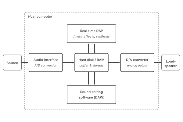
Figure 1.6. Overview of digital sound storage within a computer used for media production. The audio interface can either be a built-in feature or connected via USB, Thunderbolt, or other port. It contains the hardware for analog-digital conversion and storage onto hard disk. Some interfaces will also contain on-board synthesizers. Sound editing and processing software allows loading sounds into RAM for subsequent playback, editing, processing, etc. Some interfaces carry their own signal-processing hardware for additional processing, though a current computer manages the work unaided. Finally, digital-analog conversion occurs for eventual playback to the receiver. See also Figure 5.1.
As regards the final product of the medium, it is true that some artists never use a method for storing their art for replication at another time; it is always performed live. But with production audio, there is always a need to store the final result on a transportable and replicable medium. Digital media and streaming platforms are critical in this regard; due to the large storage requirements of visual images and audio, the evolution from physical discs to cloud delivery is what has really made modern media production flourish. Modern storage and bandwidth continue to increase, and the speed of access and capabilities are only limited by the hardware and network connection of the host device.
Playback of digital audio is complicated by the fact that there’s an infinite number of listening situations that cannot be predicted. The many different types of headphones and loudspeakers that are available all sound different, making it necessary to ascertain the influence on the final audible result. Things are made more complicated by the fact that the location of the speakers and the environment in which they are placed will influence the sound before reaching the ear of the receiver, particularly the spatial aspect of the sound. For example: sit directly between the speakers and to listen to an example of when one ear is too close to one speaker and not the other; and then to hear the intended spatial effect.
We have defined the sink or receiver as the listener’s hearing system, their immediate perceptual responses, and their higher-level cognitive processing. An audience comprises multiple receivers, each different in some way; but the original receiver is the author-sound designer-composer who has formulated the sound. This person will have a highly personal set of criteria for what sounds good, appropriate in a certain setting, etc. But listening tastes are as highly individual as people themselves, meaning that what works for the sound designer might not work for a large number of people. Whoever the target audience is, the difficulty of predicting individual taste must never be underestimated. If this were not true, there would be automatic formulas for creating hit records, although certain kinds of music are more formulaic than others, due to extensive market research of the lowest common denominator of what will be pleasing for a large audience. Despite the gratification of mass appeal, the rewards of targeting critical acclaim, cult status, or niche markets should not be discounted.
At the listener, hearing consists of both physical and perceptual transformations of the incoming sound field. A thumbnail sketch of the main features of the physical hearing system is shown in Figure 1.7. There are many books available that offer more in-depth descriptions of the physiology of the hearing system; one area that is of particular interest to those involved in computer speech recognition is the mechanics of the cochlea and the basilar membrane. The attempt to model the ear electronically is a fascinating challenge that may one day contribute to perfect speech recognition by computers.
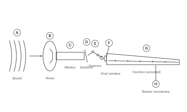
Figure 1.7. Highly simplified, schematic overview of the auditory system. See text for explanation of letters. The cochlea (G) is unrolled from its usual snail shell-like shape.
Sound (A) is first transformed by the pinnae (the visible portion of the outer ear) (B) and proximate parts of the body such as the shoulder and head. Following this are the effects of the meatus (or ear canal) (C) that leads to the middle ear, which consists of the eardrum (D) and the ossicles (the small bones popularly termed the hammer, anvil, and stirrup) (E). Sound is transformed at the middle ear from acoustical energy at the eardrum to mechanical energy at the ossicles; the ossicles convert the mechanical energy into fluid pressure within the inner ear (the cochlea) (G) via motion at the oval window (F). The fluid pressure causes frequency-dependent vibration patterns of the basilar membrane (H) within the inner ear, which causes numerous fibers protruding from auditory hair cells to bend. These in turn activate electrical action potentials within the neurons of the auditory system, which are combined at higher levels with information from the other (opposite) ear. These neurological processes are eventually transformed into aural perception and cognition, including the perception of spatial attributes of a sound resulting from both monaural and binaural listening.
That is the airborne route, and it is not the only one. Sound also reaches the cochlea straight through the bones of the skull, bypassing the outer and middle ear entirely — bone conduction. Everyone has already run the experiment. A recorded voice sounds wrong to its owner and to nobody else, because while speaking the speaker hears two things at once: the airborne sound everyone else receives, and a bone-conducted component carried through the jaw and skull from the vibrating vocal folds. Bone favours the low frequencies, so the voice heard from inside is fuller and deeper than the one a microphone captures. The recording is not thin; it is simply the half of the sound that was always being shared, arriving without the private half that usually accompanies it.
Physical and Perceptual Descriptions of Sound
In the following section, we introduce the fundamental terminology used in describing sound. These factors correspond to how we are able to identify and discriminate different sounds perceptually. In particular, we’ll look at the correspondence between the following physical and perceptual descriptions of sound:
| Physical terminology | Perceptual terminology |
|---|---|
| Frequency | Pitch |
| Intensity | Loudness |
| Spectra (& other factors) | Timbre (tone color) |
The pairing is a useful first approximation rather than an identity. Each perceptual quantity depends on more than the one physical quantity beside it — loudness varies with frequency as well as with intensity, and pitch shifts slightly with level — and a percept can be revised outright by evidence from another sense entirely. The sharpest demonstration is the McGurk effect: when a spoken /ba/ is dubbed onto video of a mouth articulating /ga/, most listeners hear neither and report “da.” Closing the eyes restores the recorded syllable at once, and opening them brings the fusion straight back — even for a listener who knows precisely what is being done. Hearing is an inference drawn from whatever evidence is available, and the eyes are part of that evidence.
Waveform Frequency
A sound waveform is defined as a time-varying disturbance of air molecules that propagates through space in three dimensions as the result of the vibration of an object at a different location from the receiver. Some disturbances repeat, and a sustained tone is periodic; most do not. Speech, noise, and the transient of a struck object are all sound, and none of them repeats. Look around: countless objects are in a state of vibration. The windows on a house when a truck drives by, the wood on a guitar when a string is plucked, the infrastructure of a building, or the branches of trees in the wind. The listener’s inner ear contains organs that vibrate in response principally to air molecule disturbance, converting these vibrations into changing electrical potentials that are sensed by the brain allowing the phenomenon of hearing to occur. Similarly, a pressure microphone contains a diaphragm that vibrates in response to the disturbance of air molecules by a sound waveform, and then converts the vibration of the diaphragm into electrical signals that can be amplified and stored. When the vibration is within the frequency range of human hearing (conventionally about 20 to 20,000 vibrations per second for a young listener with healthy hearing, with wide individual variation and an upper limit that falls with age), the waves are heard as sound waves.
Figure 1.8 shows an audio waveform as compression and rarefaction of air molecules. Two animated versions follow: one for a point source (spherical wavefronts radiating outward from a loudspeaker), and one for a line source (planar wavefronts marching down a tube). The static figure further below then samples the same disturbance at five distinct moments of time t0–t4 for inspection. In both animations, individual air molecules oscillate within their own bounded excursion — they do not propagate with the wave; the wave is the moving pattern, not the medium. Compression (denser packing, blue tint) is the positive pressure and rarefaction (sparser packing, red tint) is the negative pressure of a single waveform cycle (or oscillation) of these molecules.
Point Source — Spherical Wavefronts
A 2-D view of a longitudinal sound wave radiating outward from a loudspeaker on the left. Each dot is one air molecule. Each molecule oscillates along its radial line from the source, back and forth within a small bounded range, while curved compression (blue) and rarefaction (red) bands sweep outward through the field. Five tagged red molecules carry an explicit red excursion bar (with end-caps perpendicular to the radial direction) and a fading trail — pick any one and watch: it bounces between its two end-caps and returns to where it started, while the wavefront pattern passes through it. Drag the Speed slider to slow down, freeze (speed = 0), or reverse the wave.
Line Source — Planar Wavefronts in a Tube
A 2-D view of a longitudinal sound wave travelling rightward through a tube of air, driven by a vibrating line source (drawn as a tuning fork at the left). The wavefronts here are planar — flat sheets perpendicular to the tube — rather than spherical, because every part of the source moves in phase along its length. Each dot is one air molecule; molecules oscillate back and forth horizontally about their rest position. Four bright-yellow tracked molecules make this explicit: each has a yellow range-bar showing its excursion limits (with end-caps) and a vertical tick at its rest position, plus a fading trail. Watch one tracked molecule for a few cycles — it bounces between the two end-caps and returns to where it started, while the compression / rarefaction pattern marches rightward past it. Drag the Speed slider to slow down, freeze (speed = 0), or reverse the propagation direction.
Try this with either animation: (a) Set Speed = 0 to freeze the wave, then compare a molecule in a compression band with one in a rarefaction band — they’ve been displaced from rest spacing in opposite directions. (b) Bump Speed to 0.1× and follow a single tagged molecule with the eye: it just oscillates locally, it doesn’t travel with the wave. (c) Drag Speed negative: the wave reverses but each molecule’s motion is still purely local.
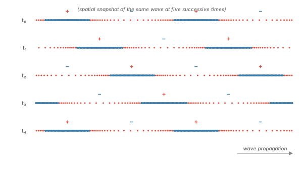
Figure 1.8. The same waveform sampled at five discrete moments of time. The + indicates compression (an increase in pressure) and the − indicates rarefaction (a decrease in pressure). The horizontal axis is position, the vertical axis is successive time slices — each row is the wave a moment later than the one above, so the “+” and “−” regions drift visibly rightward as the wave propagates.
The most common way to draw a wavelength’s oscillation is to indicate its pressure variation continuously over time, as shown in Figure 1.11. The x axis is used to indicate time, and the y axis is used to indicate negative or positive pressure about 0 (the thick line in the middle). Each vertical line is equivalent to the intervals of time t0–t4 shown in Figure 1.8.
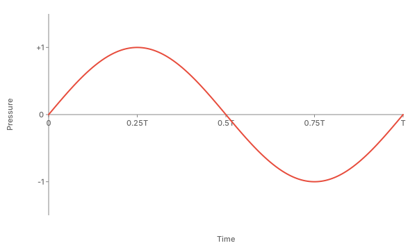
Figure 1.11. A single cycle (wavelength period) of a continuously repeating waveform (here, a sine wave) is shown as a continuous function of time on the x axis, with pressure on the y axis shown in both positive and negative directions from the center line.
An audio waveform frequency is defined in terms of the number of waveform cycles that occur during one second. Drop a rock into the middle of a lake and circles propagate outward from the point where it landed. These circles are equivalent to how sound waves travel, except in this case the medium of disturbance is water rather than air. If the number of waveform cycles that pass a single point on the lake over one second is measured, the frequency of the waveform will be calculated.

Figure 1.12. This sine wave has a frequency that is five times the frequency of the waveform in Figure 1.11.
In the waveform displays of Figures 1.10 and 1.11, we can count how many cycles occur during the time interval t0–t4 by observing the number of times the waveform repeats itself. Note that the waveform in Figure 1.12 repeats itself five times over the same time interval as shown in Figure 1.11; we would then say that the frequency of the waveform in Figure 1.12 is 5 times as high as the frequency of the Figure 1.11 waveform. Assume that each tick t is equivalent to 0.01 seconds. We use the Greek letter τ (“tau”) for the period — the time taken to complete one full wavelength — to keep it distinct from the time variable t. The frequency f is then 1 divided by the period:
f = 1 / τ
The waveform in Figure 1.11 repeats itself at t4, so one cycle has period τ = 0.04 seconds. Calculating 1/τ = 1/0.04, we obtain a frequency of 25 cycles per second (abbreviated cps). Usually, the term hertz (abbreviated Hz) is used instead of cps. Because Figure 1.12 shows a waveform with five times the frequency of the waveform shown in Figure 1.11, it has a frequency of 125 Hz.
Once digitized and displayed on the computer, most everyday acoustic waveforms are harder to analyze graphically as to their frequency. Any waveform that repeats itself indefinitely in a predictable manner is termed a periodic waveform; most periodic waveforms are obtainable only from synthesizers and audio test equipment. Figures 1.10 and 1.11 show the simplest type of periodic waveform, the sine wave. The sine wave exists in pure form only in the domain of electronically produced sound, or in theoretical discussions of sound as a means of describing real waveforms. It has a single constant frequency and amplitude that never varies. Because of these special properties, it’s one of the most basic signals used in audio synthesis, sound analysis, and even hardware testing of sound systems, as heard later in Chapter 8.
Frequencies may also be given in kilohertz (abbreviated kHz); it means the number of oscillations times 1,000 that occur within a second. For example, 1.6182 kHz (1.6182 × 1000 Hz) is the same frequency as 1,618.2 Hz.
Sine Wave Listening Examples
Now let’s listen to some sine waves. Use loudspeakers rather than headphones for these examples. Listening to very loud sine waves for extended periods of time can be very irritating and can potentially cause equipment or hearing damage if played too loud. Before starting, to verify that the sound system is working correctly. If one still doesn’t hear anything and the volume is all the way up, check out the sound set-up guidelines in the introduction or the beginning of Chapter 8.
to listen to a sine wave at 110 Hz. Nothing may be audible at all, simply because many computer sound systems are incapable of reproducing this frequency.
to listen to a sine wave at 220 Hz. The sound may sound faint because of the frequency response of the particular system.
to hear a sine wave at 440 Hz. This is the “A-440” contemporary musicians use as a tuning reference, but historic tunings varied: In Mozart’s time, A was 421 Hz; In Handel’s era, A was 422.5.
to hear a sine wave at 880 Hz. Note that the sound seems to be louder than 440 Hz. It will even be louder in the next two examples, not necessarily because of the sound system, but because our hearing system is relatively more sensitive to these higher frequencies than the ones just heard (we’ll talk about this in the section below on loudness). A warning, just to be safe:

Volume warning: The following higher-frequency sine waves may seem significantly louder. Turn down the volume before continuing.
to hear the sine wave at 1760 Hz or 1.76 kHz; notice how this example seems much louder than the previous ones.
to hear the sine wave at 3.52 kHz. This might even seem louder still.
to hear the sine wave at 7 kHz. This might seem louder or quieter, depending on the frequency response of the speakers.
Figure 1.13: Explore Frequencies
Pick a waveform, set frequency and gain, click or tap Play. The top pane shows the time-domain waveform; the bottom pane shows the log-frequency spectrum. Push the Gain past 100 % to drive the signal into hard clipping — the waveform flattens at the top and bottom, and new harmonic partials appear in the spectrum (the same distortion mechanism illustrated in Fig 2.5).
Pitch — Perceived Frequency
Many people familiar with music but unfamiliar with audio technology think of frequency in terms of pitch. But there is an important difference; frequency is a physically measurable quantity, whereas pitch refers to the perception—i.e., human interpretation—of frequency. To use a cooking analogy: a sauce can take 1, 1.25, or 4 teaspoons of salt, but the one with 4 teaspoons does not taste “four times as salty,” and the difference between 1 and 1.25 may pass unnoticed.
Generally speaking, any two frequencies that are in an octave relationship to one another are recognized as being more perceptually similar than if they were in any other relationship. Because of this, frequency perception is more logarithmic than linear. Note that on repeatedly doubling a certain audible frequency, say 100 Hz, the linear distance between each successive octave gets wider. This means that pitch perception and octave relationships are more closely logarithmic instead of linear. Correspondingly, we’re more sensitive to differences at lower rather than higher frequencies.
Music uses pitch names to describe the frequency relationships between sounds. A sound with twice or half the frequency of a given sound, which we heard previously with the sine wave examples, is termed to have an octave relationship to the other pitch. 220 Hz is an octave above 110 Hz; 880 Hz is an octave below 1760 Hz, and two octaves above 220 Hz; 220 Hz is two octaves below 880 Hz; etc. These frequencies are equivalent to the musical note A. On a piano keyboard, A3 = 220 Hz is the frequency of the A below middle C; 440 Hz is the frequency of A4, or A above middle C, an octave above the A below middle C. In fact, A 440 is widely used as a tuning reference for musical instruments — the so-called concert A. Figure 1.14 shows where these frequencies are in relationship to a piano keyboard.
Figure 1.14: Click or tap the Keys
The relationship between notes on the piano keyboard and frequency. Click or tap (or drag across) the keys to hear sustained pure tones — the spectrogram below shows their frequency content over time (low at the bottom, high at the top). The three A keys (A3 = 220 Hz, A4 = 440 Hz, A5 = 880 Hz) sit at evenly spaced heights, demonstrating that octaves are linear on a log-frequency axis. Switching the Microphone on draws the room on the same axes, so a sung note can be compared with a played one — its harmonics land in the same places, or nearly so.
Figure 1.14. Live keyboard with spectrogram. Each pure-tone note appears as a horizontal stripe at its frequency on the log-frequency vertical axis — the A keys land on evenly-spaced rows because each octave is a doubling.
Our hearing system is quite sensitive to the difference in frequency of two tones down to a particular minimum difference, called the just noticeable difference (JND). Because pitch perception is logarithmic, it depends what frequency is being considered when one asks what the JND is between two pitches, but it is generally true that the JND increases with frequency. The JND is roughly estimated for convenience’s sake to be around 1/100th of a minor 2nd interval; this is termed a cent. (A minor second is the interval between any two adjacent piano keys, black or white. For instance, B–C, C–C#, and C#–D are all minor seconds.)
Beat Frequencies
When someone tunes a stringed instrument, they play two different strings, using a pitch on one string (or a tuning fork) as a reference and all the while comparing it to the pitch of another string, which is changed in frequency by adjusting the string tension with a tuning peg. When the two pitches get close to a JND, they start to create auditory beat frequencies. The beating starts fast and then gets slower and slower as the pitch of the two strings are brought into a unison or octave relationship. Click or tap on each cell of Figure 1.15 below to listen; toggle the A/B button to hear each detuned pitch with an in-tune comparison tone (beats appear) or solo (much harder to detect the detuning).
Figure 1.15. Variation of pitch in cents around an in-tune reference. Use the A/B toggle to hear each detuning with vs without a comparison pitch — with comparison (A), the auditory beats give the deviation away; without (B), even ±10 cents is surprisingly hard to spot.
| ← sharper | in tune | flatter → | ||||
|---|---|---|---|---|---|---|
Figure 1.16: Beat Frequencies
Set two close pitches and listen to the beats. Below: the sum waveform on the left shows the slow amplitude envelope that gives beats their pulsing character; the Lissajous figure on the right plots tone 1 against tone 2 — the ellipse rotates at exactly the beat frequency, so a stationary loop = unison and a fast spin = far-from-tune.
The equivalence between pitch and frequency can become messy with real sound sources. For example, musicians commonly modulate frequency over time using a technique known as vibrato. Although the frequency is varied as much as a semitone at a rate of 3–8 Hz, a single pitch is perceived. Consider the technique of stretch tuning used by piano tuners; specifically, the relationship between the fundamental frequency of a piano string and pitch as associated with the tempered piano scale. Going up from the reference note A 440, a professional tuner will progressively raise the frequency of the strings and will tune strings progressively flat for lower pitches.
With computer audio, we’re usually not that concerned with what the exact frequency of a sound is unless we’re composing music. More important is the relative frequency. As we’ll see in Chapter 7, there are several methods available for changing the frequency of a recorded sound.
One thing the beating demonstration shows is not beating at all. Set the two tones far enough apart — the Rough preset puts them 40 Hz apart — and the slow throb gives way to a harsh buzzing that is neither one pitch nor two. The boundary being crossed is the critical band: the width of the region of the inner ear over which the two tones are still competing for the same stretch of basilar membrane. Two tones inside one critical band cannot be resolved separately, so what is heard is their sum fluctuating — slow enough and that is beating, fast enough and it is roughness. Once they are far enough apart to fall in different critical bands, the ear separates them and two distinct pitches are heard instead. The band is roughly a fifth to a sixth of its own centre frequency over most of the audio range, so it is narrow in absolute terms at the bottom of the scale and wide at the top — which is why two low notes a semitone apart sound muddier than the same interval played high.
The same limit explains masking, met later in these pages: a loud tone hides a quieter one most effectively when both fall within one critical band, and it is precisely this that perceptual codecs such as MP3 exploit when they discard what the ear was never going to hear.