Audio Basics III: Spectra, Modulation, and Phase
How complex sounds are built from simple components, how amplitude and frequency modulation shape timbre and expression, and why the phase relationship between waveforms matters.
Spectra and Harmonics
Most sound sources contain multiple vibration frequencies (“modes of vibration”) that occur when the source is activated. While a sine wave is considered technically to be a “simple” waveform, almost all waveforms in nature are in actuality “complex,” in that they contain multiple frequencies that make up the spectrum (plural, spectra) of a waveform. The reason a piano or the oboe doesn’t sound like a sine wave is because every sound source has its own unique spectrum. Click or tap each of the buttons below. Each sound source has an identical musical pitch, but a unique spectrum, allowing us to categorize each sound source as unique:
Figure 3.1. Six same-pitch samples with per-sample spectrograms. Click or tap each number to play that sample. Its spectrogram — time across, log-frequency up — draws below the button and freezes after the sample ends, so all six can be played and their spectra compared side-by-side. They share the same fundamental pitch (D3, ~147 Hz) but differ in their overtone content (timbre): each label gives a one-word character cue.
The recording process and signal processing can radically alter a sound’s spectrum. Each of the sounds below are from the same piano sound source but the spectra has been altered by digital filters. A filter is most often used in audio to alter the spectrum of a sound.
The most familiar form of spectral modification is adjusting a sound source via a tone control or a graphic equalizer. These modify the spectral balance of an input sound by selectively emphasizing some frequency components and de-emphasizing others. Figure 3.2 shows a typical graphic equalizer setting from a software editing package.
Figure 3.2: Graphic Equalizer
Ten-band graphic equalizer at standard ISO octave frequencies (31.5 Hz to 16 kHz). Drag any slider to boost or cut that band by ±12 dB. The white curve is the resulting filter response, drawn over the live spectrum of the selected audio source. Pick a preset (“disco curve,” “smiley face,” “telephone,” …) and listen as it remaps the spectral balance.
Figure 3.2. A graphic equalizer divides the audible spectrum into a fixed set of frequency bands and allows each to be boosted or cut independently. The infamous “disco curve” preset shows the canonical lots-of-bass-some-treble shape; try it on a music track to hear the spectral re-balancing directly.
Timbre
The spectrum of a sound source, along with the manner that the content changes over time, is largely responsible for the perceptual quality of timbre, sometimes referred to simply as “tone color.” Timbre is sometimes defined in terms of what it is not: “the quality of sound that distinguishes it from other sounds of the same pitch and loudness.” Everyone is innately pretty good at recognizing and distinguishing between different timbres. There’s evidence that babies can distinguish between mom’s voice and another person’s early in life. Konrad Lorenz was one of the earlier workers who found that birds inside of the egg are imprinted with their mother’s voice, or whomever happens to be making continual sounds; if a human peeps at an egg for long enough, the baby bird will recognize that human as “mom.” For example, most people recognize the sound of a friend’s car or other vehicle long before seeing it: waiting on a busy street corner, the listener hears hundreds of different vehicle sounds yet can pick out that one particular automobile, motorcycle, bicycle, or skateboard from its timbre alone.
There are still more complicated explanations for distinguishing between and identifying different timbres. For instance, some workers have found that a loudspeaker judged to look inexpensive is also judged to sound worse than one that looks expensive. Other research suggests that the following are important:
- the range between pitch and noise-like character
- the spectral envelope (the evolution of spectra over time)
- the overall rise, duration, and decay of amplitude
- small pitch changes in both the fundamental frequency and the spectra
- information contained in the onset of the sound, as compared to the rest of the sound
Luckily, we can use that most accurate measuring device, our hearing system, to make most of the distinctions that are necessary.
Partials, Fundamentals, and the Harmonic Series
Each individual frequency that makes up an individual sound’s waveform is termed a partial. The partial with the lowest frequency in a complex sound is termed the fundamental. Often, but not always, a sound’s pitch is mostly influenced by the frequency of the fundamental rather than by higher partials; in many cases the fundamental frequency has more energy than the other partials. Each of the examples heard on the previous page had identical fundamental frequencies, in terms of Hz. However, their amplitude behaved differently over time, providing another cue for timbral differences.
The simplest types of partials are called harmonics. These are vibration modes where the partials are simple multiples of the fundamental. Harmonic partials are familiar from a guitar string. A plucked string is heard at its lowest frequency; that is its pitch. Lightly touching the string at its halfway point (see Figure 3.3) sounds a tone an octave above the fundamental — the second harmonic, also called the first overtone. Touching the string so that its length is divided into a ratio of 3:2, and the pitch sounds a perfect fifth plus an octave above the fundamental; and so on. Stopping the string at different locations causes the string to vibrate in different modes. The simple-ratio divisions of the string correspond to the overtone series (or harmonic series) seen at the right of Figure 3.3.
Figure 3.3. Producing different harmonics on a guitar string by stopping the string at points corresponding to simple ratios (left); the equivalent musical pitches that make up the overtone series (right). Each harmonic row carries two narrowcasting toggles — solo (🔊) plays that harmonic and adds it to the audible mix; mute (🔇) blocks it. Hover any harmonic row to reveal a tooltip naming its musical contribution (root / fifth / major-third / minor-7th …) within the currently-sounding chord. Keyboard shortcuts: number keys 1–9 toggle mute (🔇), Shift ⇧ + 1–9 toggle solo (🔊).
An interesting phenomenon related to spectra is that of fundamental tracking, which explains how the pitch of a bass player remains audible on a small speaker incapable of reproducing that frequency. In most cases, the ear determines the pitch at the correct fundamental based on the harmonic relationship of the higher harmonics that the speaker is capable of reproducing.
Seen from the percept’s side rather than the loudspeaker’s, the same effect goes by the name virtual pitch: partials at 800, 1000, and 1200 Hz are heard as one tone at 200 Hz — a frequency present nowhere in the signal. How the hearing system arrives at it is still an open question, and two accounts remain in contention: pattern matching, which fits the resolved partials against a harmonic template, and periodicity detection, which reads the pitch from the repetition rate of the waveform itself. Both predict the bass line on the small loudspeaker; they part company on inharmonic and mistuned partials, which is where the experiments concentrate.
- Autocorrelation is the periodicity reading. Multiply the signal by a delayed copy of itself, integrate, and sweep the delay: a periodic waveform scores a peak at every whole multiple of its period, so the lag of the first strong peak gives the period and its reciprocal the pitch. Nothing in the procedure requires the fundamental partial to be present.
- The cepstrum takes the spectral route — it is the spectrum of the log magnitude spectrum, and its axis, in seconds again, is called quefrency. Because a logarithm turns a product into a sum, the harmonic comb of the excitation collapses into a single peak at the pitch period, well clear of the smooth resonance envelope that carries timbre and formants. One transform thus separates what drives a voice from what shapes it.
Figure 3.4: Build a Sound from Harmonics
Pitch (partials & nearest tempered note)
Combined waveform — the sum of all active harmonics:
Spectrum — bar height is each partial’s effective amplitude (slider position, modulated by mute 🔇 / solo 🔊):
Individual harmonics — each colored line shows one partial’s waveform and amplitude:
Keyboard shortcuts: number keys 1–9 toggle mute (🔇) for harmonics 1–9; the same keys with Shift ⇧ toggle solo (🔊). So pressing Shift ⇧+4 Shift ⇧+5 Shift ⇧+6 extracts a just-intoned major chord from a complex tone.
Tip: harmonics 1·2 give plain octave doubling, the most ancient and culturally universal sonority. Add harmonic 3 to get the power fifth (root + octave + perfect 12th), the open-fifth power chord of medieval organum and modern rock. Harmonics 4·5·6 produce a just-intoned major triad; adding the 7th gives the bluesy harmonic dominant 7th chord (its 7th sits about 31 cents flat of an equal-tempered B♭). Harmonics 5·6·7 on their own form a diminished triad, not a major chord.
Figure 3.5: Fourier Sandbox
A deeper-dive companion to the Harmonics Builder above. Each of 16 harmonics has two sliders: in polar representation they are magnitude + phase; in rectangular representation they are the sin coefficient + cos coefficient. The two representations describe the same waveform — switching is a coordinate change. In Draw edit-mode the time-domain canvas accepts mouse / touch strokes; on release the demo runs a discrete Fourier transform of the drawn waveform and writes the first 16 harmonic magnitudes & phases back into the sliders. The waveform operators (time-reversal, full / half rectification, resampling, quantizing, clipping, noise) round-trip the synthesized waveform through a sample-by-sample transform then re-DFT it back into the sliders. Each harmonic has a mute / solo pair for narrowcasting (keys 1–9); the spectrum panel can superimpose 1/nk reference envelopes; and hovering any harmonic’s column highlights its contribution across the time-domain trace, the spectrum bar, and the synthesized-waveform equation simultaneously.
Time-domain (one period)
Frequency-domain magnitude (per harmonic)
Magnitude
Phase (−180° – +180°)
Narrowcast (mute / solo) · 0–9 = mute, Shift + 0–9 = solo (0 = DC) ·
Waveform operators
Each operator transforms the current synthesized waveform sample-by-sample, then runs a real-input DFT on the result and writes the first 16 harmonic magnitudes & phases back into the sliders. The transform is therefore lossy: anything above the 16th harmonic is discarded by the DFT. Button glyphs follow the standard math shorthand: |·| = absolute value (full-wave rectify), x+ = max(0, x) — the “positive part” that clips negative excursions to zero (half-wave rectify), d/dt = numerical derivative.
Synthesized waveform
RMS · by Parseval's theorem, RMS = √(Σ aₙ2 / 2) — phases drop out of the sum, so any (mag, phase) combination with the same magnitudes has the same RMS (and the same total power).
Figure 3.5. The Fourier Sandbox — a deeper-dive companion to Figure 3.4. 16 harmonics + a DC term, toggleable polar (magnitude + phase) or rectangular (sin + cos) representation, draw-on-canvas → DFT → sliders, waveform operators (time-reversal, rectification, resampling, quantizing, clipping, noise), per-harmonic mute / solo narrowcasting (keys 0–9 mute, Shift + 0–9 solo), 1/nk reference-envelope overlays on the spectrum, and reverse hover-highlight: pointing at a column — or a term in the synthesized-waveform equation — lights up that harmonic’s contribution across the time canvas, the spectrum bar, and the equation simultaneously.
Simple Periodic Waveforms
There are other simple periodic waveforms other than the sine wave that can be produced on analog synthesizers, test equipment, and FM synthesis using an electronic oscillator. A triangle wave is composed of a fundamental frequency with partials at odd numbered multiples: 1 × the fundamental frequency f, 3 × f, 5 × f, 7 × f, etc. ( to hear a triangle wave with a fundamental at 250 Hz). A square wave (see Figure 3.6) is composed of a fundamental frequency with partials at odd numbered multiples: 1 × the fundamental frequency f, 3 × f, 5 × f, 7 × f, etc. ( to hear a square wave with a fundamental at 250 Hz). Both waveforms use only the odd harmonics, but the two fall away at very different rates. For the square wave the amplitude of each harmonic is the reciprocal of the harmonic number: given a fundamental at 250 Hz, the partial at 750 Hz has one third the amplitude, the partial at 1250 Hz one fifth, and so on. For the triangle wave the amplitudes fall off far more steeply — as the reciprocal of the square of the harmonic number, so one ninth at 750 Hz and one twenty-fifth at 1250 Hz, with every other harmonic inverted in sign — which is why a triangle wave sounds so much closer to a pure sine than a square wave does.
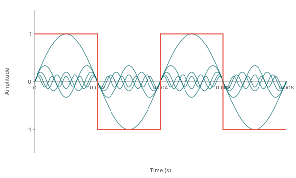
Figure 3.6. A square wave (in red) superimposed over sine waves that represent its first five (odd-numbered) partials, at 250, 750, 1250, 1750, and 2250 Hz. An actual square wave would be composed of successive odd-numbered harmonics up to the highest frequency capable of being produced by the audio system (in a digital system, almost half the sampling rate).
A sawtooth wave contains both even and odd harmonics; like the square wave, each harmonic’s amplitude is the reciprocal of the harmonic number. Figure 3.7 shows two ways of describing a sawtooth wave. In the inset, the time display of the sawtooth waveform is shown as a function of amplitude. Figure 3.7 also shows a graph of the relative amplitude of each of the first five harmonics.
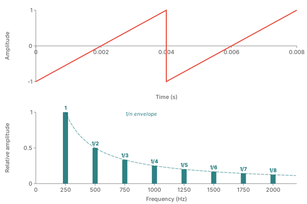
Figure 3.7. Sawtooth wave. Inset: time display with the x axis used for indicating time. Below, the frequency of each harmonic, instead of time, is shown on the x axis.
Figure 3.8: Harmonic Envelope Explorer
Set how fast the harmonics drop off. The amplitude of the n-th harmonic is 1/nk. With Sawtooth selected, every harmonic is present, so k = 1 is the classic sawtooth and k = 2 tapers toward a rounded-parabolic shape. With Square selected, even harmonics are zeroed out (a fundamental property of the square waveform), so k = 1 is the canonical square wave and k = 2 gives the same harmonic-magnitude envelope as a triangle wave (odd-only, 1/n2 rolloff) — but not the same time-domain shape: a real triangle's odd harmonics alternate sign (sin − sin / 9 + sin / 25 − …), and this demo holds all phases at zero, so the frequency-magnitude bars match a triangle's but the waveform doesn't. See Fig. 3.24 for the phase-alternation point in detail. In either base, k = 3 approaches a pure sine. The harmonic slot spacing is identical between the two waveforms — only the even bars vanish in Square — so the two spectra are directly comparable. Slider has detents at integer k. Caveat: only the rolloff magnitude changes — phases are held fixed (sin), so this is a study of how the spectral envelope shapes the time-domain waveform without phase modulation.
If the sawtooth wave is decomposed into sine wave components, a graph like that in Figure 3.9 results:
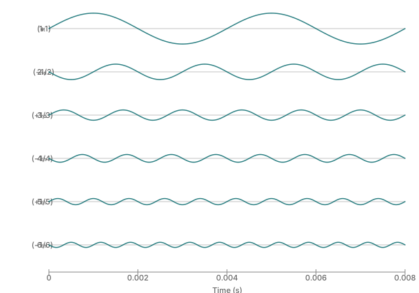
Figure 3.9. Sine wave decomposition of the first 6 partials of a forward sawtooth (fundamental 250 Hz; each partial at frequency n × 250 Hz, amplitude (-1)n+1/n). Even-numbered partials are inverted (note how each successive partial starts in the opposite direction from the previous one) — that’s what makes the partial sums in Fig 3.10 ramp up rather than down. Solo (🔊) a row (or keyboard shortcut Shift ⇧ + n) to add that synthesized sine to the audible mix; mute (🔇, or keyboard shortcut n) blocks it. Stacking multiple solos builds up successive partial sums of the sawtooth in real-time.
In Figure 3.10, we add each of the partials of the sawtooth wave progressively. Notice how the waveform looks more and more like the sawtooth shown in Figure 3.7, above. We would need to add together many more partials to get the perfect-looking sawtooth shape. Click or tap each waveform to hear it.

Figure 3.10. Partial sums of a reverse-sawtooth (falling-ramp) waveform at 250 Hz: Σ(1/n)·sin(2πn·250t) for n=1..k, with k=1 through 6. All-positive coefficients (no sign alternation) — that’s why the ramp falls and snaps back up. To get the forward sawtooth (rising ramp), alternate signs: Σ((-1)n+1/n)·sin…. Gibbs overshoot is visible at each discontinuity. Click or tap any plot to hear it.
Inharmonic Partials and Noise
The partials of a complex sound usually break down into both harmonic and inharmonic frequencies. A harmonic partial is a vibration that is related to the fundamental frequency of a vibrating medium by ratios that are either mathematically simple (e.g., 3:2) or complex (e.g., 3.14159:2). Most complex waveforms in nature contain many harmonic and inharmonic frequencies, while waveforms containing only harmonically-related tones are almost always synthetic.
Some waveforms have such a complex set of harmonics occurring at one time that it is difficult to determine where the fundamental is. For instance, to hear the sound of a gong. Notice that the low harmonic seems to fade in and then out (a kind of amplitude modulation, as we’ll discuss below).
Other waveforms might also contain what are termed noise-like components. What people mean by this is that there’s a certain amount of non-harmonic “fuzz” occurring at many frequencies. For instance, a cymbal has so many frequency components that it is difficult to state that any one is that sound’s actual pitch ( to hear the cymbal). The amount of noise-like components contained within a waveform can influence the perceived timbre of a sound significantly. Listen to the following two sounds:
to hear a violin tone played “normale” and
to hear a violin tone played “col legno.”
Normally, the bow is played against the string so that its hairs activate the natural harmonics of the violin string with significant intensity relative to inharmonic partials. In the second example the violin was played col legno, where the wood part of the bow instead of the hair is rubbed against the string. This causes the non-harmonic components to have relatively greater intensity.
Speech is comprised of both noisy and periodic vibrations. Figure 3.11 shows both noise components (sh and t) and quasi-periodic components (u) within a speech recording of the word “shut.” Try saying the “sh” portion of shut; it sounds like the white noise heard previously. Now say the “u” portion. Note that it’s possible to change the pitch of “u”, depending on how it is said ( to hear “u” pitched at different frequencies). On the other hand, the pitch of the “sh” portion cannot be changed; only its spectral balance can, by shaping the mouth differently.
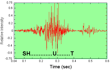
Figure 3.11. A waveform plot of the spoken word “shut.” A noise-like (aperiodic) portion for the “sh” sound precedes the more pitched “u” sound, while the “t” is transient.
For certain types of noise it is easiest to describe its frequency in a statistical manner. Figure 3.12 shows a plot of white noise, a non-periodic waveform of the type discussed earlier in Chapter 1. White noise can be thought of as the complete opposite of a sine wave: a sine wave has a single deterministic frequency with a predictable amplitude, while white noise has no deterministic frequency with random amplitudes. It has a “flat” spectrum, meaning that it contains all frequency components at equal intensity.
Another type of noise frequently used in audio applications is pink noise. Rather than containing equal power at every frequency, pink noise contains equal power within each octave.
Figure 3.12. The five “colors” of noise, ordered by spectral tilt from low-frequency to high-frequency emphasis. Left: for each color, a lag-1 return map (x[n] plotted against the previous sample x[n−1]) beside a zoomed time trace. The trace alone makes white, blue, and violet look alike once it is dense, but the return map separates them by their correlation structure: a diagonal cloud where each sample resembles its neighbor (persistent — the brown/red end), a round cloud for memoryless white, and an anti-diagonal cloud where neighbors oppose (anti-persistent — blue, and violet more tightly still). Right: the idealized spectrum on log-frequency × dB axes, where each color is a straight line of a distinct slope, so all five — including violet — are equally distinguishable: Brown / Red (1/f², −6 dB/octave), Pink (1/f, −3), White (flat, 0), Blue (f, +3), Violet (f², +6). The straight lines are what the curved, saturating time traces cannot show.
Figure 3.13: Noise Color Explorer
Tip: click or tap a preset to snap to a canonical noise color, or drag the slider to hear smooth transitions across the spectrum. The visualization shows the real-time spectrum (linear frequency axis). An RMS-makeup gain keeps overall signal power (integrated ∫|x(t)|2dt) roughly constant across the sweep — that’s pure mathematical energy, not perceived loudness. Violet will still feel louder than brown of equal energy because human hearing peaks in sensitivity around 2–5 kHz (Fletcher–Munson) — right where the violet boost is concentrated.
Look closer — amplitude distribution (Gaussian vs uniform)
The histogram in the top-right of the plot shows the noise’s amplitude distribution — how often the signal sits near each value — against the ideal Gaussian bell (amber). This is a separate property from the spectrum: “white” describes the flat spectrum, not the amplitude shape. Gaussian and uniform white are both white, have the same spectrum, and sound the same — switching here changes the histogram but not the color. Now the payoff: pick Uniform (its histogram goes flat), then drag the tilt toward brown and watch the flat histogram become a bell. Tilting toward brown makes each output sample a weighted sum of many input samples, so the Central Limit Theorem takes over — the same reason low-frequency-weighted noise in nature tends to be Gaussian whatever its microscopic origin. (Tilt toward violet instead — differencing, few samples — and it stays non-Gaussian.)
Physical intuition — the calculus ladder
Every color here is white noise tilted by repeated calculus. Integrating (accumulating) reddens the spectrum by 6 dB/octave; differentiating (differencing) blues it by 6 dB/octave. That gives a kinematic ladder for a random walker: if its position is brown (a random walk, −6 dB/8ve), then its velocity — the independent step-to-step kicks — is white (flat), and its acceleration is violet (+6 dB/8ve). Position, velocity, acceleration = brown, white, violet, each one derivative apart. Brown accumulates its steps (they pile up, so it wanders off); violet’s samples instead anti-correlate (a step up tends to be followed by a step down), so its energy sits up high. Pink and blue are the half-steps (−3 and +3 dB/8ve) — fractional integrals, with no clean integer-derivative picture. This demo realizes any of these slopes with a tilt filter (a time-domain shelving filter that shapes the spectrum as the audio streams through it), which is distinct from an FFT-based spectral method that instead transforms into the frequency domain, scales each bin, and transforms back.
A word on what exactly is tilting, since the slopes above are quoted in dB and the names are quoted as powers of f. The exponent α in 1/fα describes the power spectral density: pink is α = 1, brown α = 2, blue α = −1, violet α = −2. The amplitude spectrum carries half that exponent — pink noise has amplitude falling as 1/√f, not as 1/f. The two nevertheless give the same figure in decibels, because power is quoted as 10 log and amplitude as 20 log, so both describe pink as −3 dB per octave and brown as −6. The dB slope is −3α dB per octave in every case. It is worth holding the two apart: the exponent and the decibel figure are the same statement only once the right multiplier has been used on each.
Why pink is special: equal power per octave. White noise carries equal power per hertz, so each higher octave — twice as many hertz — holds twice the power, which is why white sounds bright and hissy. Brown dumps nearly everything into the lowest octaves. Pink (−3 dB/8ve) is the one tilt where every octave carries the same power. Because hearing works in octaves (log frequency), pink sounds perceptually even — which is why it is the standard signal for loudspeaker and room calibration, and why 1/f spectra recur so widely in nature, from flicker noise to music to heartbeats.
Amplitude Modulation (AM) and Amplitude Envelopes
Most naturally-occurring acoustical phenomena caused by a momentary excitation (the transference of energy from a drum stick, air, keyboard hammer, etc. to the vibrating object) have a characteristic where the overall amplitude builds to a maximum relatively quickly and then decays relatively slowly, although in a manner characteristic of the particular sound source. We refer to the overall pattern of amplitude change over time as the amplitude envelope of a sound.
Figure 3.14 shows an “overall” amplitude envelope of all the partials of a complex waveform, as specified on a synthesizer. Note that, like a piano, the sound does not stop when the key is released, but takes a brief moment to “die out.” In reality, each individual harmonic and inharmonic component of a natural, complex sound will have its own amplitude envelope, making the overall amplitude envelope only a rough approximation of the sound’s temporal evolution. To hear this, to hear the lowest note of a grand piano while the sustain pedal is held down; the effect is strongest on a real piano. Several very different amplitude envelopes are at work, emphasizing and de-emphasizing different harmonics over time. It is the complex interaction of these harmonics over time that gives the grand piano its unique timbral quality and makes it very difficult to synthesize. Sound designers must work very hard to avoid regularity in the short term or long term envelopes of each of a synthesized sound’s harmonics as well as its overall amplitude envelope, if a “natural” as opposed to “synthetic” character is desired.
Figure 3.14: ADSR Envelope
Adjust the four ADSR parameters with the sliders or by dragging the yellow handles directly on the envelope: A sets the attack time; S sets both the decay time (horizontally) and the sustain level (vertically); H sets the note-hold duration; R sets the release time. Click or tap Note to hear the envelope applied for the slider-set hold time. Or press and hold the Hold to play button (mouse, touch, or the Space / Enter key when it is focused) to gate the note by hand: the playback cursor climbs through attack and decay, then waits at the sustain level — for as long as the key is held — and only begins the release phase on letting go. That is the whole point of sustain: a level held for an indefinite, gate-driven time, not a fixed duration.
Figure 3.14. The ADSR (Attack-Decay-Sustain-Release) amplitude envelope. A, D, S, and R describe what happens when a key is held and then released: attack and decay shape the onset; sustain is the held level; release governs how quickly the sound dies after the key lifts. Each instrument family has a characteristic ADSR shape — the presets above sketch a few canonical ones.
to listen to the sound of a violin being plucked with the fingers (a pizzicato note). The waveform is shown in Figure 3.16. Notice how the amplitude envelope has greatest amplitude when the string is initially plucked, how the amplitude is reduced considerably after this point, and then how the sound dies away steadily as the amplitude of the vibration of the string (and its resonance within the body of the violin) diminishes. Note also how the waveform looks noisy at first, and then how periodic frequency can be detected later in time.

Figure 3.16. A waveform of a plucked violin string, along with its amplitude envelope.

Figure 3.17. The amplitude envelope of a zipper being opened.
Figure 3.17 shows the amplitude envelope of a zipper being pulled open. to listen to its sound. Note the envelope is loudest when pulling harder on the zipper, and then dies down quickly once the zipper is going smoothly. The amplitude envelope is irregular since the resistance of pulling open a zipper will also be irregular.
The importance of the attack portion of the amplitude envelope to the perception of timbre can be demonstrated in the following examples. All three are from the same sound source: a natural harmonic played on an acoustic guitar.
Attack vs. DSR — Stereo Lateralization
With stereo headphones or speakers, drag the slider to pan the attack sample to the left and the decay·sustain·release sample to the right — from mono (both centered) up to a hard split. Both samples start simultaneously on Play both, so the “bite” and the resonance can be heard separating spatially.
Tip: a guitar’s natural attack is only a few milliseconds — below the brain’s left/right fusion window (~30 ms), so even at 100 % lateralization the attack and DSR can fuse into a single percept. Toggle Slow down 4× to stretch both samples in time so the attack lasts long enough to perceive in just one ear.
The first example is the unaltered guitar harmonic. The second is only the attack portion—this is where the “bite” of the sound is produced in the excitation of the string, and is characteristic of a guitar attack. The third example is only the decay and sustain portion. Amazingly, the sound has lost any characteristic of the guitar; it has the rich content of partials and the decay of the harmonic, but without the attack, the sound is almost like a French Horn.
The amplitude envelope is a form of amplitude modulation. Multiplying the output of a digital device by a time-varying function is a form of amplitude modulation. Similarly, wiggling the volume control on an amplifier back and forth is hand-operated amplitude modulation. Amplitude modulation means “varying gain over time.” Figure 3.19 shows the amplitude modulation of a sine wave by two cycles of a triangle wave, shown below in Figure 3.18. The triangle wave oscillates at a much slower frequency than the sine wave; while the sine wave is within the audio frequency range, the triangle wave used here has a frequency of about 0.5 Hz, well below the lowest frequency of human hearing. We hear the effect of the triangle wave, demonstrated by the up-and-down ramping of the sine wave’s amplitude.
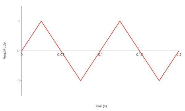
Figure 3.18. The triangle wave used for amplitude modulation in Figure 3.19.
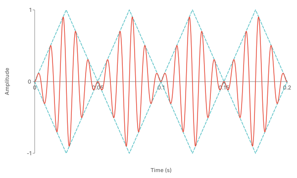
Figure 3.19. The amplitude modulation of a 100 Hz sine wave by a 10 Hz triangle wave as shown in Figure 3.18 results in a constant, synthetic amplitude envelope.
Frequency Modulation (FM)
There are two types of FM that concern us. The first is low-frequency FM, used to create vibrato (pitch modulation). The second is high-frequency FM used for synthesis. Figure 3.20 below shows a sine wave with decreasing and then increasing low-frequency modulation by a sine wave.
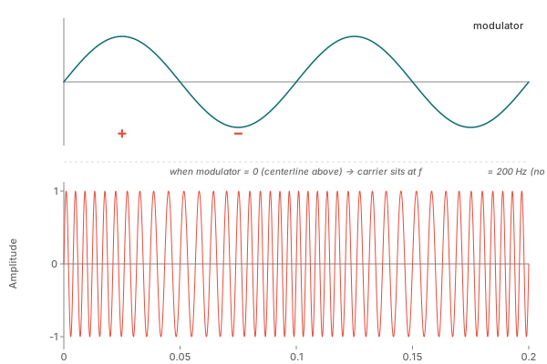
Figure 3.20. Frequency modulation. The plus signs indicate when the modulation is maximal and the minus signs when the modulation is minimal, corresponding to the peaks of the modulating sine wave.
Low-frequency modulation is usually termed vibrato. It is a variation in the frequency of a pitch above and below a fundamental pitch, usually no more than within a musical half-step. It is a feature that most instrumentalists include in their music, if it is possible to create the effect. For instance, a singer almost always uses vibrato. There are different styles of vibrato; a “wide” vibrato can sound “schmaltzy” or overly romantic, while music of the baroque era (from 1600–1750; e.g., J. S. Bach) was performed in its day with very little vibrato. Every performer uses vibrato a little bit differently, which contributes to the unique character of an individual performance.
The second example has a moderate amount of vibrato, and either no special indication or the word “normale” would be indicated in a musical score. It is interesting that in spite of the variation in frequency, we associate pitch with the center frequency of the modulation.
Figures 3.16–3.17 show the relationship between a modulating wave (the modulator) and the wave affected by it (the carrier), for both frequency and amplitude modulation. Two parameters of the modulating wave are relevant: the frequency of the modulating waveform, and the amplitude of the waveform (sometimes referred to as modulation depth). In Figure 3.21, the modulation is applied to the frequency of the carrier, while in Figure 3.22, the modulation is applied to the amplitude. Figures 3.16–3.17 use a sine wave carrier and modulator.
The two types of modulation cause quite different effects at low and medium frequencies. When the modulator goes from sub-audio to audio frequencies (the high frequency setting), spectral sidebands are produced; we hear a different timbre but not the modulator directly. The high-frequency modulation in Figure 3.21 produces relatively fewer non-harmonic partials because the modulator and carrier have simple frequency ratios. Non-harmonic frequency modulation causes a richer blend of non-harmonic partials ( to hear). Any sort of waveform can act as a modulator as well; for instance, to listen to randomly-chosen numbers (noise) as the frequency modulator. This yields a “machine computation” sound effect sometimes used in film.
Live FM demo
| FM presets | Low depth | Medium depth | High depth |
|---|---|---|---|
| Slow rate | |||
| Medium rate | |||
| Fast rate |
Tip: the presets snap the four parameters and modulator wave to canonical FM-synthesis flavors. Vibrato & Trill use sub-audio modulation (the pitch is heard to wobble). Bell, Brass, and Woodwind use audio-rate modulation that generates sidebands and entirely changes the timbre. Two-tone (Hi-Lo) siren uses a square-wave modulator so the carrier snaps between two pitches — the classic European emergency-vehicle effect.
Figure 3.21. The effect of frequency modulation (FM) of a carrier oscillator. F is the frequency control input of the oscillator; G is the gain of the oscillator. The block diagram on top updates live as the controls below are changed, or click or tap any preset. For a deeper-dive companion, Sirens & FM makes these presets nine points on a continuous plane — drag across it to hear a siren’s wail collapse into a bell’s timbre as one number crosses the 20 Hz border. Well below that border, where a repeating pattern is counted rather than heard as a pitch, lies the territory of the Rhythm Playground.
Live AM demo
| AM presets | Low depth | Medium depth | High depth |
|---|---|---|---|
| Slow rate | |||
| Medium rate | |||
| Fast rate |
Tip: Tremolo/Slow tremolo/Chopper use sub-audio modulation rates (the volume is heard to wobble or pulse). Once the modulator rate climbs into the audible range, what was a tremolo turns into ring modulation — the carrier’s spectrum sprouts sum- and difference-frequency sidebands and the timbre changes entirely.
Figure 3.22. The effect of amplitude modulation (AM) of a carrier oscillator. F is the frequency control input of the oscillator; G is the gain of the oscillator. The block diagram on top updates live as the controls below are changed, or click or tap any preset.
Waveform Phase
In addition to frequency and amplitude, the phase of a waveform is a fundamental concept for describing sound. A waveform’s phase has to do with its “starting time” relative to another waveform. It also refers to the relative onset of a group of partials within a complex sound.
For example, consider a loudspeaker with a “woofer” for low frequencies and a “tweeter” for high frequencies. Loudspeakers often use a “crossover” filter to split a signal into two frequency bands—high and low. Now consider what happens when a square wave is played through the system. If we move the tweeter closer or farther away relative to the woofer, the high frequencies will have a different phase relationship to the low frequencies.
Figure 3.23 shows two identical sine waves in terms of frequency and amplitude, but one waveform is offset in its phase relative to the other. Waveform B is delayed relative to waveform A by a period of time equivalent to a quarter period (90°) of its wavelength, which is 0.001 seconds (abbreviated s), or 1 millisecond (abbreviated ms).
Figure 3.23. Two 250-Hz sine waves, A and B. Drag the delay slider and watch the correlation swing from +1 (in phase) through 0 (90°) to −1 (180°) and back — while the coherence stays pinned at 1, because no matter the delay B is still a phase-shifted copy of A at the same frequency. Then dial in some noise on B: coherence drops too, since B is no longer a purely linear function of A. The X-Y panel on the right is the Lissajous view — A plotted against B: in phase it collapses to a diagonal line, at 90° it opens into a circle, at 180° it becomes the opposite diagonal. So the figure’s shape tracks the correlation: a collapsed line means ±1 (its slope — up or down — gives the sign), a full circle means 0. The more open the loop, the nearer the correlation is to zero. Adding noise frays the loop into a band — the visible face of falling coherence.
- Correlation is the normalized time-domain inner product. For unit-amplitude sinusoids at the same frequency, the cross-correlation at zero lag is cos(φ). With φ = 90°, the integrals of cos × sin over an integer number of cycles cancel exactly: correlation = 0. Slide one wave by 1 ms (the lag that matches the delay) and it jumps to 1.
- Coherence, γ2(f) = |Sxy(f)|2 / (Sxx(f)·Syy(f)), is taken in the frequency domain after computing each signal's spectrum. The phase term lives in the complex cross-spectrum but gets removed by taking the magnitude squared. So for the same pair of sine waves, γ2(250 Hz) = 1 regardless of how delayed B is relative to A.
Relative phase between two signals, as measured here, is one of several senses the word carries. A further one is phase velocity — the speed at which a crest advances through space, which need not match the speed of the packet the crest belongs to. The bonus page Phase & Group Velocity separates the two, and connects them to the frequency-dependent group delay of a filter.
When listening to a steady periodic waveform, it is usually very hard to distinguish between a version with all of the harmonics “in-phase” and one with some of them shifted — even though the two look quite different on an oscilloscope. Figure 3.24 shows two waveforms consisting of the first six harmonics of a triangle wave. The blue and red waveforms are identical except that every other harmonic is out-of-phase in the red version.
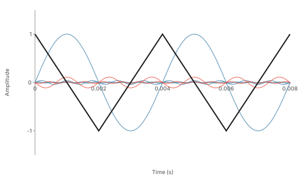
Figure 3.24. Triangle wave with in-phase (blue) and out-of-phase (red) harmonics.
Although the two waveforms in Figure 3.24 look different, they sound identical: to listen to the in-phase version, and to listen to the out-of-phase version. For steady tones such as these, the ear is far more sensitive to the magnitude spectrum than to the phase relationships among the harmonics, which is why the two versions sound so alike. That is a claim about this particular kind of stimulus, though, and it should not be stretched into a general one: relative phase between components does become audible under other conditions — with low fundamentals, with widely-spaced components, over headphones, and with transient rather than sustained material — and there is a published experimental literature documenting exactly that. Three separate things are worth keeping apart. Absolute phase and absolute polarity — the inversion of an entire signal — are one thing; relative phase is the alignment among a sound’s own components, which is what this figure varies; and a system’s phase response is how much delay it imposes at each frequency. “Linear phase” refers to the last of these — a constant group delay, so that every frequency is delayed by the same amount of time — and whether it is audible in a given loudspeaker or filter is a different question from the demonstration above, which does not settle it.
On the other hand, relative phase is a very significant issue for an audio system. Phase becomes an issue in production audio when mixing waveforms electronically with an audio mixer, or when mixing waveforms in the air as occurs with two-channel loudspeaker playback. In these cases we have a situation where either constructive or destructive interference can occur. Consider the addition of two in-phase sine waves together. This is the same as multiplying the waveform by 2; each instantaneous value of the waveform sums constructively such that the resulting waveform has twice the amplitude. But summing each instantaneous value of a sine wave with another that is 180° out-of-phase gives zero amplitude (see Figure 3.25).
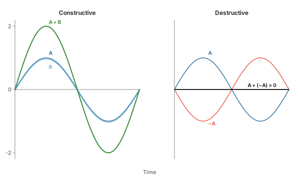
Figure 3.25. Constructive and destructive interference. The blue waveform is an in-phase sine wave. By adding this waveform to an in-phase copy of itself, the green waveform with twice the amplitude would result (constructive interference). But if the blue waveform were added to a 180° out-of-phase copy of itself (the red waveform), destructive interference results (represented by the black waveform with zero amplitude).
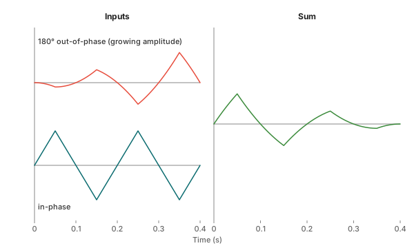
Figure 3.26. Click or tap any of the three plots to hear its waveform: the upper-left out-of-phase triangle (with growing amplitude), the lower-left in-phase triangle, or the right-hand sum where destructive interference builds as the two are mixed.
The following example shows an extreme case of how destructive interference occurs when signals are out-of-phase. The lower waveform on the left of Figure 3.26 is an in-phase triangle wave. The upper waveform at the left is the same triangle wave, 180° out-of-phase, with a steadily increasing amplitude envelope; eventually it reaches the same amplitude as the lower waveform. At the right side of Figure 3.26 is the result of adding the two waveforms on the left. In this example, the destructive interference increases as a function of the amplitude of the out-of-phase waveform.
Destructive interference can also occur when mixing waveforms in the air, for instance, from two stereo loudspeakers. Listen carefully to the next two examples with the head between the stereo loudspeakers currently in use with this website.

Volume warning: Verify the volume level before playing the following phase examples.
Stereo Polarity Sandbox
Pick any waveform and toggle between parallel wiring (both channels in phase, the normal case) and crossed wiring (right channel inverted, +180° phase). With the head between two stereo speakers, the parallel version locks to a stable center image; the crossed version smears the image and gets thinner because the two channels cancel along the center line. The diagram on the right shows the speaker wiring; the canvas plots L and R waveforms so the inversion is visible.
Listen with stereo speakers, head between them. Crossed/out-of-phase audio cancels along the center line; headphones don’t reveal the effect the same way (each ear hears only one channel, so there’s no air-mixing).
The in-phase triangle wave should create a stable image localized in-between the speakers; the out-of-phase version should sound split between two locations in the speakers, and sound less loud in one speaker. If the opposite occurs, the speakers are wired out-of-phase; reverse the leads on one of the speakers. In Chapter 8 there are additional tests for determining loudspeaker phase and details on how to reverse the phase of the loudspeakers.
To summarize, the relative phase of harmonic components within a single waveform is inaudible, but the relative phase of two waveforms mixed in either air or electronically can result in significant changes in the audio communication chain, and therefore must be taken into account.