Audio Basics II: Intensity and Loudness
How we measure waveform intensity using peak and RMS values, the decibel scale for relative and absolute levels, and the perceptual experience of loudness.
Intensity
We have shown how the frequency of a waveform is measured in terms of the variation in pressure over a unit of time of air molecules; i.e., the number of waveform periods (cycles) that occur over one second. What determines the literal intensity of the waveform and its perceived loudness is the degree of sound pressure. Our hearing system is designed to discriminate between both different frequencies and intensities of sound. A sound wave carries energy as it propagates; the power of a waveform for a given area is the intensity of the waveform (mathematically, watts/meter²). Loudness is defined as the perceived magnitude of intensity; as with pitch and frequency, there’s a “human element” of interpretation that doesn’t follow physical measurements.
Graphically, the amplitude of a periodic waveform can be observed by noting the height, or peak value of a periodic waveform on the y axis. Figure 2.1 shows two cycles of a 1 kHz sine wave: the blue waveform peaks at an amplitude of 1, twice the amplitude of the red waveform, which peaks at 0.5. Amplitude and intensity are not interchangeable here: intensity goes as the square of pressure amplitude, so twice the amplitude corresponds to four times the intensity. The numbering scale used on the y axis graphs the maximum possible range of amplitudes for each sample, within the range −1 to 1.
Figure 2.1: Peak, Peak-to-Peak, RMS
Two periodic waveforms of the same shape are shown: blue at full amplitude (peak = 1), red at half amplitude (peak = 0.5). The green double-headed arrow measures the full peak-to-peak swing of the blue wave. The orange dashed lines mark the blue wave’s RMS — the equivalent constant amplitude that delivers the same average power. RMS depends on shape: 1/√2 (≈ 0.707) for sine, 1 for square, 1/√3 (≈ 0.577) for sawtooth and triangle. Pick a waveform and the dashed lines move accordingly. Press Play to hear the blue wave at the chosen frequency.
Figure 2.1. Peak, peak-to-peak, and RMS amplitude of a periodic wave. RMS depends on the waveform’s shape, not just its peak.
This is one way to represent the maximum dynamic range of a system; intermediate values are represented in the graph (but not internally on the computer) as floating-point numbers—a number with a value to the left and to the right of the decimal point. On a computer, intensity can be described in arbitrary units (e.g., ±1) for computational purposes, since we are measuring a relative level of a sound sample. We can also use what is termed the signed integer sample value, with numbers ranging from -32767 to 32767. These represent the numbers used internally with 16-bit quantization (see discussion in Chapter 6). Most waveform editing software offers a choice between sample values or percentage of dynamic range used.
Intensity can be described in terms of the peak-to-peak value of the waveform according to a scale (green lines in Figure 2.1). The intensity of a periodic waveform can be easily observed in this way, but non-periodic waves such as those in Figure 2.2 are more difficult to describe in this way. In such cases intensity is measured by computing the root mean square (RMS) value. This is obtained by squaring all of the instantaneous values of a waveform over a given period, taking the average of that value, and then obtaining the square root of that number. For instance, the peak value of the blue waveform in Figure 2.1 is 1, but the RMS value would be .707. In Figure 2.2, the RMS value, in terms of the relative intensity -1 to 1 and in terms of relative dB is shown.
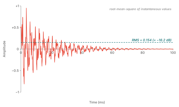
Figure 2.2. The RMS value is obtained of a given period of a waveform by squaring all of its instantaneous values; taking the average of that value; and then obtaining the square root of that number. Using the 20log10 formula, we can obtain the RMS dB value.
Relative dB
In Figure 2.2, we see the conversion of the RMS level to a value expressed in relative dB. It is convenient to express the maximum dynamic range of a digital system with floating-point numbers in the interval -1 to +1. Using the following equation for relative dB gives a scale where maximum intensity is 0, and lesser values have negative numbers, much like on a VU meter:
relative dB RMS = 20 log10 (RMS value)
Given the RMS intensity value of 0.154 in Figure 2.2, we obtain −16.2 dB RMS. Multiplication of a waveform by 0.5 results in a reduction of 6 dB (for instance, a 0 dB RMS waveform multiplied by 0.5 becomes a −6 dB RMS waveform). This type of relative dB measurement is typically used in computer audio software “change gain” controls.
Here is an example of relative dB levels. First set the playback volume to a low setting, just loud enough that the 0 dB level is still audible. Then click or tap each of the buttons in succession to hear the sound attenuated progressively by 6 dB. Probably only the first couple of buttons will be audible before the sound dies out completely. Repeat the exercise but with the volume towards maximum (taking care that the external amplifier is not too loud). The entire intensity range of sounds should now be audible.
We don’t have any idea how intense the sound pressure will be at the listener’s ears, since there are many different elements in the communication chain between the information stored in the computer and the listener. A digitized sound can be represented as a floating point number 0.565, or a signed integer 28363, but we’ll never know the actual sound level since we have no idea what levels are involved with the playback system.
dB Sound Pressure Level (SPL)
The absolute, as opposed to relative, intensity of a sound wave is expressed as the dB sound pressure level, abbreviated dB SPL. The decibel is a logarithmic way of expressing a ratio, but the two quantities take different coefficients: a ratio of powers or intensities is 10·log10(I1/I2), while a ratio of pressures or amplitudes is 20·log10(p1/p2). The factor of 20 is not a separate convention: intensity goes as the square of pressure, and squaring inside a logarithm doubles it. For dB SPL specifically, the ratio is taken against a fixed reference — the lowest audible intensity recognizable by an ideal hearing system (e.g., a newborn’s) — so an absolute level can be reported:
dB SPL = 20 log10 ( p1 / p2 )
For dB SPL, p2, or 0 dB, is equivalent to a reference sound pressure of 20 µPa — 0.00002 newtons/meter². This relates incoming levels to a previously-agreed upon reference level of 0 dB that is roughly equivalent to the threshold of hearing.
The way to measure p1 in the equation above is with a dB SPL meter. This is a useful device for measuring absolute as opposed to relative sound levels of an audio system, a neighbor’s dog barking, or the aircraft flying overhead at night. To perform some of the audio tests in Chapter 8, an inexpensive one is worth obtaining (or a calibrated SPL meter app on a smartphone).
Many books have charts of typical SPL levels. Outside rural or wilderness settings, the quietest level typically encountered is around 30 dB SPL (in a recording studio). A conversation runs about 60 dB SPL, instrumental music can reach 100 dB SPL, and things get painful around 120 dB SPL. The measurement of dB SPL is also influenced by different possible weighting scales and the distance from where the measurement was taken to the sound source. In non-reflective environments, SPL falls 6 dB with each doubling of distance.
Volume Controls and Arbitrary Scales
Intensity adjustments are most familiar in the form of a volume control (properly, a potentiometer). For instance, the following represents increments of waveform intensity, from 0–7, that are typical of operating system control panels. Click or tap each of the buttons, in sequence:
Now compare these levels to levels that we know are 6 dB apart. Set the volume to maximum, and then play 7 (above) and 0 dB (below). They’re at the same intensity. But what about 6 and -6 dB? 3 and -24 dB?
The 0–7 scale used here echoes the coarse volume scales of early personal-computer operating systems (classic Mac OS, for instance, exposed only eight steps for adjusting the volume of system sounds, alerts, and other sources such as games or audio playback). Modern operating systems offer finer granularity — macOS uses sixteen steps (with a sixteen-step fine adjustment for sixty-four effective stops), iOS sixteen, Windows a hundred — but the principle is the same. Like the numbers printed on the volume control of a portable audio player, this particular scale represents an arbitrary system: the numbers don’t really mean anything except that there’s a relative loudness increase with larger numbers. The number system doesn’t help when trying to make something sound “twice as loud.” For example, click or tap 2 and then click or tap 4. Does 4 sound twice as loud as 2? Now click or tap 2 and then 6. Does 6 sound three times as loud as 2? More than likely not.
Since there’s a chain of events within an audio system that can change the overall level, we’ll never have an absolute idea of the final loudness at the end of the chain. If the output of the computer is connected to a stereo system or powered loudspeakers, there’ll be separate volume controls at least two locations: on the computer and on the audio system. Additionally, many audio interfaces have their own output gain controls that scale the overall output voltage, and the particular hardware and drivers installed can affect the final level.
Loudness
Loudness is the perceptual correlate of intensity; they’re not the same thing, although many people get them confused. The loudness of a waveform varies widely as a function of frequency. Furthermore, the relative loudness across frequency is different at loud playback levels, compared to quiet ones. For sine waves, equivalent loudness contours can be looked up on an equal loudness contour graph (see Figure 2.3). Each contour on the graph traces the sound pressure level needed at each frequency to hold one constant loudness. The curves are drawn from ISO 226:2003 over the range that standard defines, 20 Hz to 12.5 kHz, and the lowest one is the threshold of hearing — which dips below 0 dB SPL around 3–4 kHz, where the ear canal's resonance makes hearing most acute. For instance, a tone at 60 dB SPL is not as loud at 200 Hz as it is at 4000 Hz. Not surprisingly, the majority of the frequency content of speech (approximately 100 Hz–4 kHz) is within the part of the curves that show maximal sensitivity. Note that with the lower dB SPL contour lines, sensitivity to low frequencies is lower than with higher frequencies, but at higher SPLs, the contours are more linear. The loudness and “bass boost” buttons found on consumer audio equipment are designed to compensate for this decrease in sensitivity to low frequencies at low sound pressure levels.
Figure 2.3: Equal-Loudness Contours
Click or tap Play, then drag the teal dot around the chart. Its x-position sets the test-tone frequency (log scale, 20 Hz–20 kHz); its y-position sets the nominal playback level in dB (the chart’s axis; the browser cannot know the true SPL at the ear, which depends on the output device, its volume setting, and the headphones). Try dragging along a single contour — the tone should stay at roughly constant loudness even as the dB SPL changes radically. Then drag vertically at a fixed frequency, or horizontally at a fixed dB SPL, to hear how dramatically perceived loudness depends on frequency. Headphones recommended; start with playback volume low.

Frequency: 1.00 kHz · Level: 40 dB SPL · Nearest contour: ≈ 40 phon
Figure 2.3. Equal loudness contours (after Fletcher & Munson / ISO 226). Each contour is a constant loudness level in phons, and shows how the sound pressure level required to reach that loudness varies with frequency. Furthermore, the relative loudness across frequency is different at loud playback levels, compared to quiet ones. For sine waves, equivalent loudness contours can be looked up on an equal loudness contour graph (see Figure 2.3). Each contour on the graph traces the sound pressure level needed at each frequency to hold one constant loudness. For instance, a tone at 60 dB SPL is not as loud at 200 Hz as it is at 4000 Hz. Not surprisingly, the majority of the frequency content of speech (approximately 100 Hz–4 kHz) is within the part of the curves that show maximal sensitivity. Note that with the lower dB SPL contour lines, sensitivity to low frequencies is lower than with higher frequencies, but at higher SPLs, the contours are more linear. The loudness and “bass boost” buttons found on consumer audio equipment are designed to compensate for this decrease in sensitivity to low frequencies at low sound pressure levels.
Try this: (a) Drag the dot along the 40‑phon contour — it dips to about 36 dB SPL near 3–4 kHz, where the ear is most sensitive, and climbs to roughly 64 dB SPL at 100 Hz, yet the perceived loudness barely changes. (b) Drag vertically at 30 Hz: one has to climb 30–40 dB before the bass even becomes audible — the “loudness” and “bass boost” buttons on consumer audio gear exist to compensate for exactly this. (c) Drag horizontally at a fixed 50 dB SPL: the 4 kHz region jumps out as much louder than 100 Hz even though the dB SPL hasn’t changed.
Two units are in play here, and they are easy to confuse. The phon measures loudness level: a sound is at 60 phons if it is judged as loud as a 1 kHz tone at 60 dB SPL. It is a decibel scale in disguise, and it inherits the decibel’s awkwardness — 80 phons is not twice 40. The sone measures loudness itself, as a ratio: two sones is twice as loud as one, four is twice again. The two are pinned together at 1 sone = 40 phons, and above about that level each further doubling of sones costs roughly 10 phons — which is the familiar rule that ten decibels buys a doubling of loudness, stated the other way round.
Behind that rule lies the oldest result in psychophysics. Weber observed that the smallest detectable change in a stimulus is a roughly constant fraction of it, not a constant amount: at a whisper, near 30 dB SPL, about a decibel must be added before the change is noticed, and at a shout, near 100 dB, it is still about a decibel — though in absolute terms that second decibel is ten million times more power than the first. Fechner turned the observation into a scale by counting those steps up from the threshold of hearing, giving sensation proportional to the logarithm of the stimulus, which is exactly the shape of the decibel. Stevens later showed the logarithm is not quite right and that a power law fits the judgements better: loudness grows as intensity to roughly the power 0.3. That number is the same rule again — ten times the intensity raised to 0.3 is almost exactly two — and it is why the decibel, invented for engineering convenience, happens to track hearing as closely as it does.
Dynamic Range and Clipping
The two most important aspects of intensity in the process of capturing and transferring audio material can be described as either having “not enough” or “too much” signal intensity. Figure 2.4 illustrates the problem of matching dynamic ranges between different mediums. If the intensity of a waveform is too small, all or some portion of its energy will be masked by the noise floor of the system or the environment. If external speakers are present, it’s possible to exceed the dynamic range and push the signal into distortion, by overdriving the speaker cones or the built-in amplifiers. This also involves the levels used with recording equipment, which is covered in more detail in Chapter 5. Note in Figure 2.4 that the noise floor of most playback environments (except a recording studio) is around 40 dB.

Figure 2.4. Illustration of waveform dynamic range. The teal bars show the natural acoustic range and the windows captured by various digital recording formats; the orange bar is a typical playback environment’s noise floor. The red downward arrow marks the clipping ceiling — signal driven above this gets distorted by the medium. The gray upward arrow marks the noise floor — signal below it is masked by ambient noise. The recording engineer’s job is to keep the signal between the two. Another means of accomplishing this is via compression (see Chapter 7).
When the intensity of a waveform goes beyond the electrical tolerance of any part of a circuit, distortion in the form of clipping results. The peaks of the waveform are “flattened” at the level where they exceed the maximum dynamic range of the audio system. This act of clipping introduces additional harmonic partials to the spectrum — entirely new frequencies created by the non-linearity. In some cases this is desirable, for instance with certain electric guitar sounds or other electronic instruments.
Figure 2.5: Hard-Clipping a Periodic Source
A selectable source waveform (sine, square, sawtooth, or triangle) is fed through a variable-gain stage and a hard clipper at ±1. The spectrum pane plots the magnitude at the fundamental and its harmonics (1f, 2f, 3f, …) — every periodic source has all its energy there. With a sine source at Drive = 1.0×, the wave passes through untouched: a single spectral spike at the fundamental. Raise Drive past 1.0 and the peaks flatten, the waveform morphs toward a square, and an odd-harmonic series (3rd, 5th, 7th, …) sprouts following a 1/n envelope. Other source waves already carry harmonics, which clipping reshapes further. Click or tap Play, then sweep Drive to hear and see the distortion appear in real-time.
Figure 2.5. A selectable source waveform (sine, square, sawtooth, or triangle) driven through a hard-clipper. Top pane: time-domain waveform (dashed red lines mark the ±1 clip thresholds). Bottom pane: spike spectrum at the harmonic frequencies 1f, 2f, 3f, …, log-spaced. With a sine source, an odd-harmonic series appears only once Drive exceeds 1.0; other source waves already contain harmonics, and clipping reshapes their spectra further.
Try this: (a) Start with Drive = 1.0 and confirm the spectrum is a single spike at the fundamental. (b) Slowly raise Drive past 1.0 and watch the 3rd-harmonic spike rise first, then the 5th, 7th, … in the predicted 1/n ratio. (c) Push Drive to ~6× and the waveform is nearly a square wave; the spectrum should show only odd harmonics (no even harmonics — that’s a consequence of the symmetric clip). (d) Tune Frequency low (~80 Hz): the harmonic spacing on the log axis is now wide enough for individual partials to be counted by eye.